Bilevel Differentiable Optimization

Introduction

In a previous post, we saw that we can leverage PyTorch’s autograd.Function API to create custom backward functions for any operation, for which we’d like to produce gradients via backpropagation. However, our motivating example was a bit contrived: we implemented a custom differentiable ELU, but that’s something that already exists within the PyTorch API.

In this post, we’ll tackle a more interesting use case for custom backward functions: differentiating though an inner optimization problem. We’ll see how to formalize this problem mathematically (for a simple case) and then we’ll solve it using custom backward functions.

References

This post is based on materials created by me for the CS236781 Deep Learning course at the Technion between Winter 2019 and Spring 2022. To re-use, please provide attribution and link to this page.

Motivation

Deep neural networks are powerful, but they are a rather blunt and general tool. Although they can, in theory, approximate any function, many problems have some clear structure that we can exploit. In such cases, we might turn to a more classical approach of modeling the problem as a discrete or continuous, constrained or unconstrained optimization problem, and using any number of available solvers to obtain a numerical solution. No deep learning needed.

Optimization problems

A general way to formulate an optimization problem is,

In this formulation, is the optimization variable. We’re trying to find the value of that minimizes the objective , where must be in a feasible set of allowed values. The feasible set is defined by the functions and , which are inequality and equality constraints, and by the domain (which can define e.g. whether must be an integer). The objective and constraints can be defined with parameters , , , which are fixed and simply control the shape of the problem.

There are many examples of problems that can be formulated as optimization of this form: portfolio allocation, task assignment, job scheduling, knapsack problems, ML algorithms such as support vector machines, and many more.

What if we have a structured optimization problem, but want to solve it in the context of a larger learning problem? For example, we might want to make the optimization problem itself amenable to learning, i.e. learn its parameters (not variables), and then solve it with an existing solver, i.e. find the optimal variable values given the learned parameters. The solution of the optimization problem can then be an input to another part of the deep neural network, as if it were the output of any other layer.

This is a powerful idea. It means we can essentially embed an optimization problem in a neural network, and train the entire thing end-to-end. Let’s see how we might achieve this.

Problem formulation

We’ll now make the idea of differentiating through an optimization problem mathematically concrete. To keep it from being too dense, we’ll focus on a simple un-constrained continuous optimization problem. This means that and that there are no and . However, the technique below can also be applied to a constrained optimization via its KKT conditions.

We want to solve an inner optimization problem as part of our model (a deep neural network), such that the parameters of the inner problem are also learned as part of the end-to-end optimization of the entire model. The figure below provides a visualization of what we wish to achieve.

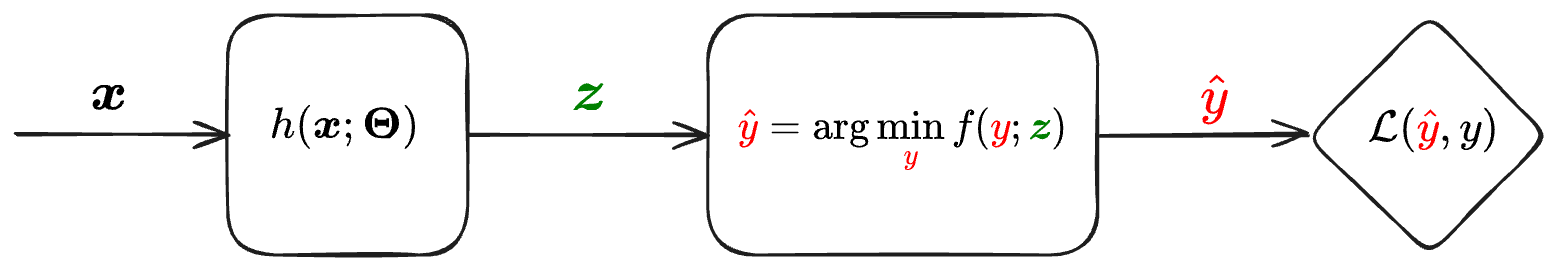
For simplicity, the figure depicts a setup where there are no additional deep learning layers after the optimization layer, though in practice there could be. We’ll refer to this new component as an “argmin layer”. Now we need to find out how we can actually train a network that contains such a layer.

Differentiating end-to-end

Training the network depicted in the figure in supervised way means we’re given datapoints , and we’re trying to find an optimal set of parameters , such that:

Notice that we essentially have one optimization problem inside another, and therefore this type of setting is also known as bilevel optimization.

From the perspective of the inner problem, is “fixed” and represents the parameters of the problem. From the perspective of the outer problem (end-to-end training), we’re optimizing to reduce the final loss, which depends on the solution of the inner optimization. We can essentially view this entire model as learning to parameterize the inner task.

How can we train such a model end-to-end via backpropagation?

Recall that for backpropagation to work, each component in the computation graph needs to implement a backward-pass function. Here’s a quick recap about what this entails (see also more details in a previous post).

Recap: The backward pass

Suppose we have a component in our computation graph that computes , where are inputs and are the learned parameters. In the forward-pass of this component, we simply need to compute .

In the backward pass, we receive an input , i.e. the gradient of the downstream loss w.r.t. to our component’s output . Then we use the chain rule to compute the gradient of the loss w.r.t. our inputs: , and . Notice that all we need to know is how to compute the derivatives of w.r.t. its arguments/paramteters. These derivatives are each a Jacobians matrix, which depends solely on the definition of our component.

Coming back to our diagram, we can see that in order for our argmin layer to be part of a computation graph, we must find a way to calculate the following vector-Jacobian product (VJP):

Once we have , we can continue back-propagating the gradient to the components that come before the argmin layer, which means we can train the whole network end-to-end. Note also that is actually simple to compute: it just depends on the loss function, which we can assume is known and differentiable (e.g. a squared-error loss for regression). The key, therefore, is computing the Jacobian .

But how can we calculate when is the solution of an optimization problem?

The Jacobian of the argmin layer

We can derive the expression for our required Jacobian from first principles, based on a Taylor approximation near the optimum.

To begin, we’ll assume that . Since is a minimizer of the function , the necessary optimality condition must hold:

In other words, the gradient of is zero at because the function has a local minimum there.

Now consider that is also a function of , and imagine that we perturb by a tiny . Assuming the function is “well-behaved”¹, the new minimum won’t be too far away because is tiny. So, after perturbing by , we’ll get a slightly different minimizer, . We can therefore write another optimality condition as,

How can we further expand the expression on the left? if we think of as just another function, then we need to know its value at a point infinitesimally close to the point .

To approximate this value, we can use a first-order Taylor expansion for around the point :

Although this is a first order expansion, our function , is already a derivative, so we get second-order derivative terms in each direction. Notice that this is an approximation (): we ignore the higher-order terms because we assume them to be very small if are very small.

Since (based on our original optimality condition), we can rearrange to obtain:

We’ll denote the Hessian as and mixed second derivatives as . We can then write the above simply as , and this yields,

The equation above means that we found a linear relationship between the change in the minimizer, , and the change in the argument value, . This linear relationship must be, by definition, related to the gradient of w.r.t. . As a simple intuition, think of the slope of a linear function, e.g. . The slope (also the gradient), is the linear relationship between the input and the output .

In fact, one way to define the gradient is that it’s the unique vector such that,

where is the standard inner product, i.e. . In other words, the gradient is by definition the vector that produces this linear relationship between an input perturbation and output perturbation. See the box below for more details.

The extrinsic definition of the gradient

For a scalar function where , the standard way to define its gradient at is via the vector of its partial derivatives, i.e.,

However, there exists an equivalent, “extrinsic” definition. The extrinsic definition states that the gradient of at a point is the unique vector such that for any unit vector ,

where is the directional derivative operator in direction :

A directional derivative is the rate of change of a multivariate function when its input moves along a given direction. A partial derivative is a special case, where the direction is one of the standard basis vectors.

Based on the extrinsic definition, projecting onto the gradient produces the directional derivative in direction .

If we now write our expression for an inner product, we have

This means that, by definition, we found that our gradient is simply

Note that is a Hessian, so it’s symmetric and we can drop the transpose.

Computing the vector-Jacobian product

Equipped with the gradient of the argmin objective, we can write the expression for the VJP that allows us to back-propagate over the argmin layer:

Since there’s a matrix inversion involved, applying this formula as-is might be numerically challenging. Therefore, we’ll split this calculation into two steps:

1. Calculate : Instead of inverting , can equivalently solve the linear system . We can solve it in a least-squares optimal sense so that the solution is still defined even if the matrix is not invertible.
2. Based on the solution, calculate .

Finally, we now have a way to implement such an inner-optimization layer:

1. Forward pass: Compute the optimal solution of the inner problem, either with a some solver or even a closed-form expression.
2. Backward pass: Calculate using the two-step procedure described above.

Implementation

Helper functions

Before implementing the argmin layer, we need some helpers.

First, let’s implement a function to calculate an approximated least-squares solution to a linear system of equations . The built-in torch.solve() only supports a square matrix A, so we’ll use a singular value decomposition (SVD) to obtain a least-squares solution in a more general case. The approach below “inverts” by computing the reciprocal of its singular values, making sure to clip very small values to maintain numerical stability.

def solve_ls(
    A: Tensor,
    b: Tensor,
    abs: float = 1e-6, # absolute tolerance
    rel: float = 1e-6  # relative tolerance
) -> Tensor:
    # Solves the system A x = b in a least-squares sense using SVD
    U, S, V = torch.svd(A)
    th = max(rel * S[0].item(), abs)
    # Clip singular values
    Sinv = torch.where(S >= th, 1.0 / S, torch.zeros_like(S))
    return V @ torch.diag(Sinv) @ (U.transpose(1, 0) @ b)

Here’s a quick test for our linear system solver:

from sklearn.datasets import make_regression
from sklearn.preprocessing import StandardScaler
 
dtype = torch.float64
torch.set_default_dtype(dtype)
 
# Create a simple regression problem
N, D = 1000, 20
 
X, y, w_gt = make_regression(
    n_samples=N, n_features=D, coef=True, random_state=42, bias=10, noise=1,
)
X = StandardScaler().fit_transform(X)
 
X, y, w_gt = [ torch.from_numpy(t).to(dtype) for t in [X, y, w_gt] ]
 
# Solve it and check the solution is close to the ground-truth
w_hat = solve_ls(X, y)
assert torch.allclose(w_hat, w_gt, rtol=0.1, atol=0.1)

Two other helper functions we’ll need are for concatenating and flattening multiple tensors together, and then reversing this operation.

In the formulation we used, we considered only one variable vector, , one parameters vector, , and moreover we treated them both as 1d vectors. However, when implementing deep neural networks, we deal with many different parameters tensors, virtually all of which high-dimensional.

For this example, we’ll deal with the case of one variable tensor (of any shape) and any number of parameter tensors (of any shape). It’s simple to use the approach here to extend to multiple variables as well. The following helpers will allow us to treat either of these as 1d tensors so that, for example, we’ll be able to compute regular 2d Hessians for them.

def flatten(*z: Tensor):
    # Flattens a sequence of tensors into one "long" tensor of shape (N,)
    # Note: cat & reshape maintain differentiability!
    flat_z = torch.cat([z_.reshape(-1) for z_ in z], dim=0)
    return flat_z
 
def unflatten_like(t_flat: Tensor, *z: Tensor):
    # Un-flattens a "long" tensor into a sequence of multiple tensors of arbitrary shape
    t_flat = t_flat.reshape(-1) # make sure it's 1d
    ts = []
    offset = 0
    for z_ in z:
        numel = z_.numel()
        ts.append(
            t_flat[offset:offset+numel].reshape_as(z_)
        )
        offset += numel
    assert offset == t_flat.numel()
    
    return tuple(ts)

Quick test for flatten/unflatten:

t1, t2 = torch.randn(3, 5), torch.randn(2, 4)
t_flat = flatten(t1, t2)
assert t_flat.shape == (t1.numel() + t2.numel(),)
 
t1_, t2_ = unflatten_like(t_flat, t1, t2)
assert torch.allclose(t1, t1_)
assert torch.allclose(t2, t2_)

Now, finally, we’re equipped to write an autograd.Function which implements differentiable optimization!

Argmin layer

Assume that the optimization problem we wish to solve is defined by some arbitrary objective function, specified directly as a python function obj_fun. The objective function is evaluated on a vector-valued optimization variable (a tensor y) and parameters (tensors z).

We need to implement a differentiable layer that:

• Minimizes this objective in the forward pass, returning the optimal value of y.
• Produce gradients w.r.t. the parameters z in the backward pass.

Here’s the API corresponding to this:

class ArgMinFunction(autograd.Function):
    @staticmethod
    def forward(ctx, obj_fun, y, *z):
        return argmin_forward(ctx, obj_fun, y, *z)
    
    @staticmethod
    def backward(ctx, grad_output):
        return argmin_backward(ctx, grad_output)

Forward pass

To implement the forward pass, we need a general-purpose solver that can optimize our objective function. We’ll use the L-BFGS algorithm (a quasi-Newton method, which we discussed in previously), since it’s general, works well for reasonably sized problems, and has a PyTorch implementation. In practice, you may use other solvers too. Note that for this approach to work, we must assume that obj_fun is itself differentiable, i.e. implemented with PyTorch differentiable operations.

from torch.optim import LBFGS
 
def argmin_forward(ctx, obj_fun, y, *z):
    # Calculates forward pass though argmin layer: returns y_argmin
    # obj_fun(y, *z) evaluates the optimization objective we want to minimize
    
    # Note: solving for y, treating the z's as constants
    optimizer = LBFGS(params=(y,), lr=0.9, max_iter=1000)
 
    # Closure for LBFGS which evaluates the loss and calcualtes
    # gradients of the variables.
    def _optimizer_step():
        # zero gradients
        y.grad = torch.zeros_like(y)
            
        # evaluate loss
        f = obj_fun(y, *z)
        
        # Calculate gradients
        # Note: not calling backward() because we don't want to compute
        # gradients for anything except y
        δy = autograd.grad(f, (y,), create_graph=False)[0]
        y.grad += δy
        
        return f
 
    # Solve the optimization problem - will evaluate closure multiple times until convergence
    f_final = optimizer.step(_optimizer_step,)
    y_argmin = y # Note: y was modified in place
 
    ctx.save_for_backward(y_argmin, *z)
    ctx.obj_fun = obj_fun
 
    return y_argmin.detach()

There are some important and interesting subtleties in this implementation:

• The closure pattern: Some torch optimizers, such as L-BFGS, need to re-evaluate the objective function multiple times per step. We provide the optimizer with a function (the “closure”) that it can call repeatedly. This function needs to:
  • Compute the loss (the objective function value, which should be minimized).
  • Update the gradient of the loss w.r.t. the optimization variables.
• The optimizer then uses the gradient that was updated within the variables to update their value each time the closure is invoked. This is why y gets modified in place.
• Using autograd.grad directly instead of backward(). Usually, the latter is used to update the gradients on all tensors that were involved in a loss computation. However, in this case we only want to compute a gradient for y, and not for the *z tensors since we treat them as fixed parameters of the objective function. By using autograd.grad() we can limit the gradient calculation to y alone.
• Saving y_argmin for later within the context object (ctx). In the backward pass, we’ll need to compute the Hessians at the optimal value of y produced by the optimizer (the local minimum).

Backward pass

For the backward pass, we’ll implement the two-step procedure shown above, to calculate . Remember that we need to calculate the Hessians of our objective function, i.e. and . Luckily, autograd can calculate this, using a second automatic differentiation. The only complication is the shapes of and , but we’ll flatten them with our helpers so that the Hessians are 2d.

from torch.autograd.functional import hessian
 
def argmin_backward(ctx, grad_output):
    y_argmin, *z = ctx.saved_tensors
    obj_fun = ctx.obj_fun
    
    flat_y = flatten(y_argmin)
    flat_z = flatten(*z)
    
    # Wrap objective function so that we can call it with flat tensors
    def obj_fun_flat(flat_y, flat_z):
        y = unflatten_like(flat_y, y_argmin)
        zs = unflatten_like(flat_z, *z)
        return obj_fun(*y, *zs)
    
    # Compute the Hessians on flattened y and z
    H = hessian(obj_fun_flat, inputs=(flat_y, flat_z), create_graph=False)
    Hyy = K = H[0][0]
    Hyz = R = H[0][1]
 
    # Now we need to calculate δz = -R^T K^-1 δy
    # 1. Solve system for δu: K δu = δy
    δy = grad_output
    δy = torch.reshape(δy, (-1, 1))
    δu = solve_ls(K, δy) # solve_ls(A, b) solves A x = b
 
    # 2. Calculate δz = -R^T δu
    δz_flat = -R.transpose(0, 1) @ δu
    
    # Extract gradient of each individual z
    δz = unflatten_like(δz_flat, *z)
    δy = torch.reshape(δy, y_argmin.shape)
    
    return None, None, *δz  # backward's outputs must correspond to forward's inputs

Notice that we return None, None, *δz. The backward function must return a value for each input of the forward function, so these three values correspond to obj_fun, y, *z. The gradient for obj_fun is obviously None, since it’s not a tensor and isn’t part of any computation graph. The gradient returned for y is also None, however. This is because the optimal value, y_argmin does not truly depend on the input y through any differentiable computation. It was obtained directly from an arbitrary optimization algorithm.

Combining into an autograd.Function

To use these functions, we must wrap them in a autograd.Function. Previously, we saw that this allows us to call Function.apply() which invokes the forward function, while also inserting the backward function in the computation graph.

class ArgMinFunction(autograd.Function):
    @staticmethod
    def forward(ctx, obj_fun, y, *z):
        return argmin_forward(ctx, obj_fun, y, *z)
    
    @staticmethod
    def backward(ctx, grad_output):
        return argmin_backward(ctx, grad_output)

Let’s run a quick test for argmin_forward: Can we reasonably solve the simple regression problem from before?

# Define a simple linear regression objective with l1 and l2 regularization
# (just to test more than one z)
def obj_fun(w: Tensor, l1: Tensor, l2: Tensor):
    loss = torch.mean((X @ w - y)**2)
    reg1 = l1 * torch.mean(torch.abs(w))
    reg2 = l2 * torch.mean(w ** 2)
    return torch.sum(loss + reg1 + reg2)
 
# Optimization variable - init to random noise
w = torch.randn_like(w_gt)*0.1
w.requires_grad = True
 
# Optimization problem parameters
l1 = torch.randn(1, 1, requires_grad=True)
l2 = torch.randn(1, 1, requires_grad=True)
 
# Function.apply() invokes the forward pass
w_hat_argmin = ArgMinFunction.apply(obj_fun, w, l1, l2)
 
assert torch.allclose(w_hat_argmin, w_gt, rtol=0.2, atol=3)
w_gt-w_hat_argmin

tensor([-1.2346e+00,  4.1897e+00, -9.6076e-02, -2.3082e-02, -3.0409e-01,
        -1.0217e-03, -1.3882e+00, -2.1605e-02, -3.8375e-02,  9.3112e-03,
        -6.9765e-01, -5.1266e-01, -2.2289e-02, -2.3652e-02,  5.7396e-03,
         7.6026e-01, -1.8786e-02,  1.3196e-01,  4.3375e-05, -3.2390e-03],
       grad_fn=<SubBackward0>)

As a test for argmin_backward: Do we get gradients on our s ?

loss = torch.mean(w_hat_argmin)
print(f'{loss=}\n')
 
# Before backward: z (l1 & l2) gradients should be None
print(f'{w.grad=}')
print(f'{l1.grad=}')
print(f'{l2.grad=}\n')
 
loss.backward()
print(f'{w.grad=}')
print(f'{l1.grad=}')
print(f'{l2.grad=}')

loss=tensor(25.6968, grad_fn=<MeanBackward0>)

w.grad=tensor([-6.7178e-05, -3.6865e-05,  3.4647e-05, -6.1958e-02, -1.0752e-05,
        -2.8637e-03,  3.7755e-06, -6.1995e-02, -6.9965e-05, -1.8564e-05,
        -6.2705e-05,  9.4835e-05, -6.1887e-02,  1.0211e-06, -4.7480e-05,
        -5.3427e-05,  3.1789e-05,  1.1999e-04,  4.7791e-04, -7.2800e-02])
l1.grad=None
l2.grad=None

w.grad=tensor([ 0.0499,  0.0500,  0.0500, -0.0120,  0.0500,  0.0471,  0.0500, -0.0120,
         0.0499,  0.0500,  0.0499,  0.0501, -0.0119,  0.0500,  0.0500,  0.0499,
         0.0500,  0.0501,  0.0505, -0.0228])
l1.grad=tensor([[-0.0196]])
l2.grad=tensor([[-1.3549]])

Using the argmin layer in a model

To demonstrate how to use our ArgMinFunction in the context of a model, we’ll tackle a time-series prediction problem, by applying linear regression on a learned, non-linear representation of the inputs.

We’ll implement the following model:

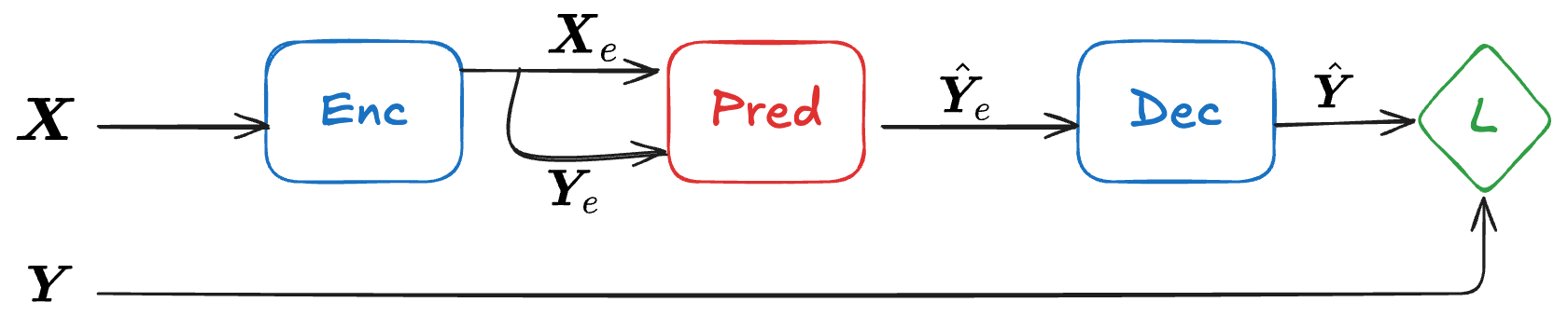
1. The encoder and decoder will be simple 1D CNNs.
2. The encoder calculates some non-linear embedding of the input, while the decoder maps an embedding back to the input space.
3. The predictor applies linear regression to fit optimal weights for predicting the last part of the embedding, from the first part, (“post-diction”):
   1. Postdiction:
   2. Prediction: where is the last part of the embedding with the same length as .

Data loading and pre-processing

Let’s load some data: We’ll use a open dataset from Kaggle, containing 12 years of daily stock price data from equities included in the Dow Jones Industrial Average (DJIA).

You can obtain this dataset here.

import pandas as pd
import numpy as np
import matplotlib.dates as mdates
from datetime import datetime
 
df = pd.read_csv("DJIA_30/all_stocks_2006-01-01_to_2018-01-01.csv.gz", compression='gzip')
df.shape

(93612, 7)

# Plot some stocks
stock_names = ["AAPL", "GOOGL", "MSFT", "AMZN"]
 
fig, ax = plt.subplots(1, 1, figsize=(12, 6))
ax.xaxis.set_major_locator(mdates.YearLocator())
ax.xaxis.set_major_formatter(mdates.DateFormatter('%Y'))
ax.xaxis.set_minor_locator(mdates.MonthLocator())
for stock_name in stock_names:
    df_stock = df[df['Name'] == stock_name]
    df_stock_dates = [datetime.strptime(d,'%Y-%m-%d').date() for d in df_stock['Date']]
    ax.plot(df_stock_dates, df_stock['Close'], label=stock_name)
ax.set_ylabel('Close Price ($)'); ax.legend();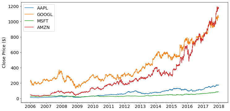

We need some minimal processing to make the data useable:

1. Split the data into segments of a fixed number of days.
2. Split each secment into a BASE () and a TARGET ().
3. Split all segments into a training and test set.

SEG_LEN = 40
SEG_BASE = 30
SEG_TARGET = SEG_LEN - SEG_BASE
 
# Filter out only selected stocks
df = df[df['Name'].isin(stock_names)]
# Split into segments of SEG_LEN days
X = torch.tensor(df['Close'].values, dtype=dtype)
X = X[0:SEG_LEN*(X.shape[0]//SEG_LEN)]
X = torch.reshape(X, (-1, 1, SEG_LEN)) # adding channel dimension
 
# Train-test split
test_ratio = 0.3
N = X.shape[0]
N_train = int(N * (1-test_ratio))
idxs = torch.randperm(X.shape[0],)
X_train, X_test = X[idxs[:N_train]], X[idxs[N_train:]]
 
# Split out target segment at the end
X_train, Y_train = X_train[..., :SEG_BASE], X_train[..., SEG_BASE:]
X_test, Y_test = X_test[..., :SEG_BASE], X_test[..., SEG_BASE:]
 
print(f"{X_train.shape=}\n{Y_train.shape=}\n\n")
print(f"{X_test.shape=}\n{Y_test.shape=}")

X_train.shape=torch.Size([210, 1, 30])
Y_train.shape=torch.Size([210, 1, 10])
X_test.shape=torch.Size([91, 1, 30])
Y_test.shape=torch.Size([91, 1, 10])

We can now visualize some random BASE and TARGET pairs.

np.random.seed(42)
fig, ax = plt.subplots(1, 1, figsize=(12, 6))
idx_perm = np.random.permutation(range(N_train))
for i in range(10):
    ax.plot(range(SEG_BASE), X_train[idx_perm[i], 0, :])
    ax.plot(range(SEG_BASE, SEG_LEN), Y_train[idx_perm[i], 0, :])
ax.axvline(x=SEG_BASE, color='k', linestyle=":", linewidth="5")
ax.grid();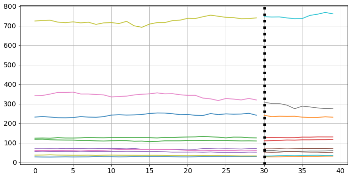

To make it easier to use this data in a PyTorch training loop, we’ll wrap the processed data in a TensorDataset and use a PyTorch DalaLoader to create batches from this dataset.

from torch.utils.data import TensorDataset, DataLoader
 
BATCH_SIZE = 8
 
dl_train, dl_test = [
    DataLoader(TensorDataset(X, Y), batch_size=BATCH_SIZE, shuffle=True)   
    for X, Y in [(X_train, Y_train), (X_test, Y_test)]
]

Model implementation

Both the encoder and decoder will use the same model, a 1D CNN. Just for fun, we’ll use the custom differentiable ELU layer (ELUCustom) that we implemented in the previous post.

class EncDec(torch.nn.Module):
    def __init__(self, channels=[1, 4, 8], out_nl=True):
        super().__init__()
        layers = []
        channel_pairs = zip(channels[:-1], channels[1:])
        for in_channels, out_channels in channel_pairs:
            layers.extend([
                
                torch.nn.Conv1d(
                    in_channels, out_channels, kernel_size=5, padding=2, bias=True
                ),
                
                ELUCustom(alpha=0.5),
                
                torch.nn.BatchNorm1d(num_features=out_channels, affine=True),
            ])
        if not out_nl:
            layers = layers[:-1]
            
        self.layers = torch.nn.Sequential(*layers)
        
    def forward(self, x):
        return self.layers(x)

enc = EncDec(channels=[1, 4, 8], out_nl=True)
enc

EncDec(
  (layers): Sequential(
    (0): Conv1d(1, 4, kernel_size=(5,), stride=(1,), padding=(2,))
    (1): ELUCustom()
    (2): BatchNorm1d(4, eps=1e-05, momentum=0.1, affine=True, track_running_stats=True)
    (3): Conv1d(4, 8, kernel_size=(5,), stride=(1,), padding=(2,))
    (4): ELUCustom()
    (5): BatchNorm1d(8, eps=1e-05, momentum=0.1, affine=True, track_running_stats=True)
  )
)

Test encoder forward pass:

x0, y0 = next(iter(dl_train))
print(f"{x0.shape=}\n")
print(f"{enc(x0).shape=}\n")

x0.shape=torch.Size([8, 1, 30])
enc(x0).shape=torch.Size([8, 8, 30])

Next, our prediction layer will use the custom ArgMinFunction to solve an optimization problem during the forward pass. Recall from the above definitions:

• The predictor uses linear regression to fit optimal weights for predicting the last part of the embedding, from the first part, (“post-diction”), and then predicts the next (unknown) part of the embedding:
  1. Postdiction:
  2. Prediction: where is the last part of the embedding with the same length as .

class PredictorArgMinLayer(torch.nn.Module):
    def __init__(self, in_features: int, out_features: int):
        super().__init__()
        self.prediction_len = in_features - out_features
        self.prediction_target_len = out_features
        
        # We'll train both W and lambda
        self.w = torch.nn.Parameter(torch.randn(
            self.prediction_target_len, self.prediction_len, requires_grad=True,
        ))
        self.reg_lambda = torch.nn.Parameter(torch.tensor([1.], requires_grad=True))
    
    @staticmethod
    def obj_fun(w: Tensor, x: Tensor, y: Tensor, reg_lambda: Tensor):
        # Objective function performing linear regression
        xw = torch.matmul(x, w.T)
        loss = torch.mean((xw - y)**2)
        reg = reg_lambda * torch.mean(w ** 2)
        return torch.sum(loss + reg)
        
    def forward(self, x):
        # Postdiction
        # X = | ------ X_e ------ | -- Y_e -- |
        x_post = x[..., :self.prediction_len] # X_e
        y_post = x[..., self.prediction_len:] # Y_e
        w_opt = ArgMinFunction.apply(self.obj_fun, self.w, x_post, y_post, self.reg_lambda)
        
        # Prediction
        # X = | --------- | ------ Z_e ------ |
        x_pred = x[..., -self.prediction_len:] # Z_e in the text
        
        return torch.matmul(x_pred, w_opt.T)

We now have all the pieces required to create the full model architecture, with an encoder, predictor, and decoder.

from typing import List
 
class EncPredictorDec(torch.nn.Module):
    def __init__(
        self, in_features: int, postdiction_length: int,
        encoder_channels: List[int], decoder_channels: List[int]=None
    ):
        super().__init__()
        
        if decoder_channels is None:
            decoder_channels = list(reversed(encoder_channels))
            
        self.enc = EncDec(encoder_channels, out_nl=True)
        self.dec = EncDec(decoder_channels, out_nl=False)
        self.pred = PredictorArgMinLayer(in_features, postdiction_length)
        self.postdiction_length = postdiction_length
        
    def forward(self, x: Tensor):
        # Calculate embeding
        x_emb = self.enc(x)
        
        # Postdict then predict
        y_hat_emb = self.pred(x_emb)
        
        # Decode back to input space
        y_hat = self.dec(y_hat_emb)
        return y_hat

Training

It’s finally time to train! Here we define the “outer” optimizer which performs the end-to-end optimization. We’ll also demonstrate how to employ simple a simple decaying learning rate schedule.

torch.manual_seed(42)
 
# Instantiate our model
model = EncPredictorDec(
    in_features=SEG_BASE, postdiction_length=SEG_TARGET,
    encoder_channels=[1, 4, 8, 16]
)
print(model)
 
# Define a regression loss for end-to-end training
loss_fn = torch.nn.MSELoss()
 
# Crete the optimizer for end-to-end training
optimizer = torch.optim.AdamW(model.parameters(), lr=1e-4, eps=1e-5)
 
# Create a scheduler to decay the learning rate each epoch
scheduler = torch.optim.lr_scheduler.ExponentialLR(optimizer, gamma=0.9)

EncPredictorDec(
  (enc): EncDec(
    (layers): Sequential(
      (0): Conv1d(1, 4, kernel_size=(5,), stride=(1,), padding=(2,))
      (1): ELUCustom()
      (2): BatchNorm1d(4, eps=1e-05, momentum=0.1, affine=True, track_running_stats=True)
      (3): Conv1d(4, 8, kernel_size=(5,), stride=(1,), padding=(2,))
      (4): ELUCustom()
      (5): BatchNorm1d(8, eps=1e-05, momentum=0.1, affine=True, track_running_stats=True)
      (6): Conv1d(8, 16, kernel_size=(5,), stride=(1,), padding=(2,))
      (7): ELUCustom()
      (8): BatchNorm1d(16, eps=1e-05, momentum=0.1, affine=True, track_running_stats=True)
    )
  )
  (dec): EncDec(
    (layers): Sequential(
      (0): Conv1d(16, 8, kernel_size=(5,), stride=(1,), padding=(2,))
      (1): ELUCustom()
      (2): BatchNorm1d(8, eps=1e-05, momentum=0.1, affine=True, track_running_stats=True)
      (3): Conv1d(8, 4, kernel_size=(5,), stride=(1,), padding=(2,))
      (4): ELUCustom()
      (5): BatchNorm1d(4, eps=1e-05, momentum=0.1, affine=True, track_running_stats=True)
      (6): Conv1d(4, 1, kernel_size=(5,), stride=(1,), padding=(2,))
      (7): ELUCustom()
    )
  )
  (pred): PredictorArgMinLayer()
)

Let’s also create a helper that implements a single epoch of the training loop:

from tqdm.auto import tqdm
 
def run_epoch(model, dl, epoch_idx, max_batches, train=True):
    desc = f'Epoch #{epoch_idx:02d}: {"Training" if train else "Evaluating"} '
    losses = []
    pbar = tqdm(dl, desc=desc)
    for i, (x, y) in enumerate(pbar):
        y_pred = model(x)
        loss = loss_fn(y, y_pred)
        
        if train:
            optimizer.zero_grad()
            loss.backward()
            optimizer.step()
        
        losses.append(loss.item())
        pbar.desc = desc + f"[loss={loss.item():.3f}]"
        if max_batches and i >= max_batches:
            break
    pbar.desc = desc + f"avg. loss = {np.mean(losses)}"
    pbar.update()

And now we can run it as follows.

num_epochs = 1
max_batches = None
 
for epoch in range(num_epochs):
    run_epoch(model, dl_train, epoch, max_batches, train=True)
    with torch.no_grad():
        run_epoch(model, dl_test, epoch, max_batches, train=False)
    scheduler.step()

Conclusion

In this post, we derived a method for differentiating through the solution of an unconstrained optimization problem, enabling us to embed an “argmin layer” within a neural network and train the whole thing end-to-end.

The key insight is that we don’t need to differentiate through the solver itself. Instead, we used the optimality conditions at the solution to obtain an expression for the Jacobian required for backpropagation through the argmin.

In practice, we saw how to solve the inner problem in the forward pass, in a way that could work for any choice of solver. Then, we computed gradients in the backward pass by solving a linear system involving the Hessian at the optimum.

Our time-series example was admittedly somewhat contrived. Ridge regression has a closed-form solution, so an implicit differentiation approach is overkill. The real power of this approach emerges when the inner problem has constraints, non-convex structure, or no analytical solution. In such cases, the same implicit differentiation idea applies, but using KKT conditions instead of just the gradient optimality condition.

I think this topic showcases the generality and power of frameworks such as PyTorch autograd, which are becoming very useful additions to include in a researcher’s computational toolbox. Hopefully, this post provided useful insights regarding both the theoretical and practical aspects of differentiable optimization.

Footnotes

1. This is a hand-wavy way of saying that the function is Lipschitz-continuous. A Lipschitz continuous function is bounded in how much its output can change when changing the input. This means the function must be smooth in some sense, i.e. it can’t “jump” too much for small changes of the input. A function is -Lipschitz continuous if there exists a constant such that for any ↩