Introduction
Convolutional Neural Networks (CNNs) have become the backbone of modern computer vision, offering an efficient way to process images with deep neural nets, without requiring either classical image feature engineering.
In this post, we explore how CNNs overcome the limitations of fully-connected networks, especially when it comes to handling high-dimensional image data. We’ll review the core building blocks—convolutional and pooling layers—and see how they work together to extract increasingly complex features from raw inputs.
We’ll also discuss practical aspects of network design, including fully convolutional architectures and the role of residual connections in deep networks. My aim with this walkthrough/tutorial style post is to provide a mix of intuitive insights, working pytorch code, and some formal definitions where needed, to help understand the core ideas behind CNNs and how they really work.
References
This post is based on materials created by me for the CS236781 Deep Learning course at the Technion between Winter 2019 and Spring 2022. To re-use, please provide attribution and link to this page.
Some images used here were taken and/or adapted from the following sources:
- Deep Learning, Goodfellow, Bengio and Courville, MIT Press, 2016
- Fundamentals of Deep Learning, Nikhil Buduma, Oreilly 2017
- Deep Learning with Python, Francios Chollet, Manning 2018
- Stanford cs231n course notes by Andrej Karpathy
- Long, J., Shelhamer, E., & Darrell, T. (2015). Fully convolutional networks for semantic segmentation. In Proceedings of the IEEE conference on computer vision and pattern recognition.
- Canziani, A., Paszke, A., & Culurciello, E. (2016). An analysis of deep neural network models for practical applications.
- He, K., Zhang, X., Ren, S., & Sun, J. (2016). Deep residual learning for image recognition. In Proceedings of the IEEE conference on computer vision and pattern recognition.
- A Comprehensive Introduction to Different Types of Convolutions in Deep Learning, Kulun Bai
- Sebastian Raschka, https://sebastianraschka.com/
- https://github.com/vdumoulin/conv_arithmetic
The limitations of MLPs for image classification
In a recent post we discussed MLPs, and saw that they are a powerful and general model which can in principle approximate any function.
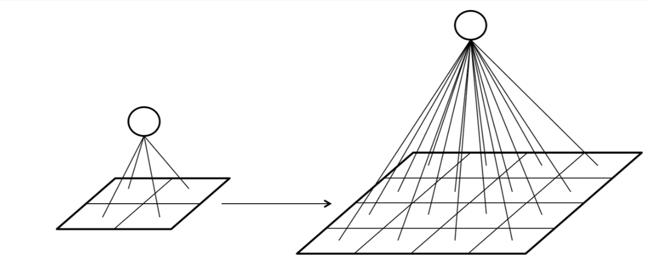
In its first layer, an MLP must connect to each of the input features.
More precisely, every single neuron in the MLP’s first layer must connect to each input feature. So if we have
If the input is an image, and we naïvely treat each pixel as an input feature, the number of parameters would increase quadratically with image size due to this connectivity. For example,
- A tiny 28x28 MNIST image would require 784 weights per neuron in the first layer.
- A modest color 1000x1000x3 color image would already require 3M weights, per neuron.
A huge number of parameters greatly increases risk of overfitting. For example, below is the effect of the number of parameters on the decision boundary of an MLP. We can see how the decision boundary becomes more complex and starts to fit the training data exactly as the number of parameters grows.
-
With 1 hidden layer, 3, 6 and 20 neurons
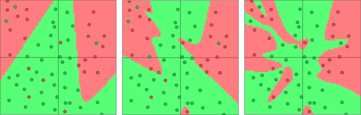
-
With 1, 2 and 4 hidden layers, 3 neurons each

Another issue with connecting each neuron to a specific set of pixels is that the these are not stable features. For example, a small translation in the image would completely change the values of specific pixels, and thus to input so most neurons. However, clearly this is not a different image and it should not be treated as such.
![]()
The classical machine-learning approach is to use feature engineering: we could apply some fixed yet arbitrarily complex transformations to the input images to extract various properties and then feed those properties as inputs to the MLP. However, with images, features are notoriously difficult to engineer.
Here we’ll see a more modern deep-learning approach: by using an architecture that’s suited for images, we can learn the feature-extraction transformations together with the task itself (e.g. classification). We’ll see that deep learning will allow us to learn hierarchical, non-linear transformations directly from the input data without requiring any feature engineering.
Convolutional Layers
A convolutional layer has a fixed number of parameters, regardless of the input size (height and width of the image) 1. Put simply, it achieves this by re-using the same parameters on different parts of the input.
We’ll explain how convolutional layers work in using three different perspectives, from the most non-formal to the most formal.
Structural perspective
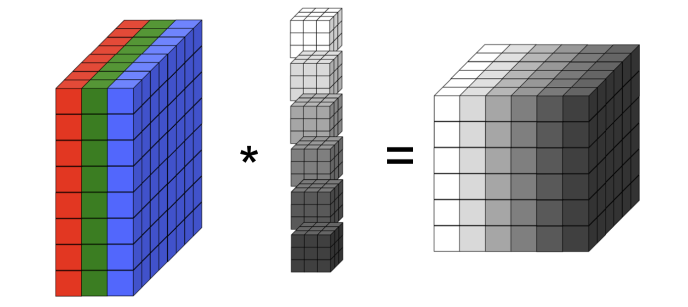
Just for intuition, a convolutional layer can be viewed as a composition of neurons, just like in an MLP, but with three important distinctions.
-
The neurons can be thought of as stacked in a 3D grid (instead of 1D).
-
Neurons at the same depth in the grid (represented here by color) share the same learned parameters (e.g.
). 
-
Each neuron is local, i.e. it’s connected only to a small region of the previous layer’s output (represented here by location). However, despite being spatially local, it operates on all channels of its input layer.
Note
It should be emphasized that this is not how convolutional layers are implemented in practice. The point is merely to provide an intuitive way to compare them to the familiar fully-connected layers.
Filter-based perspective
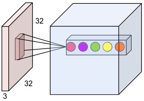
Imagine sliding a
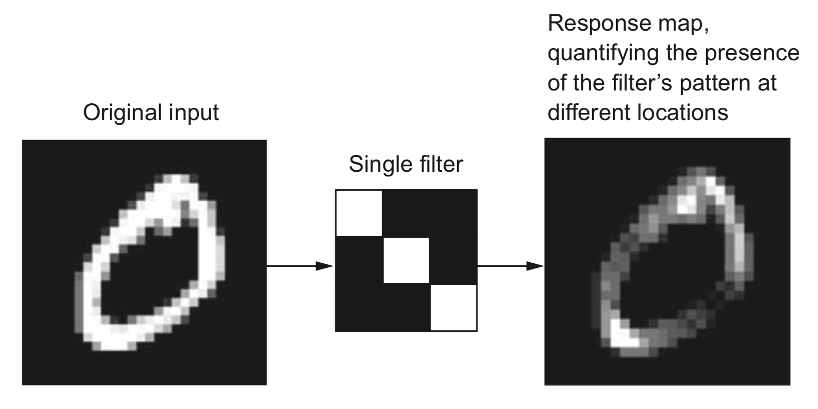
We have just computed the convolution between the filter and the image.
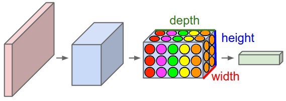
Next, imagine we have a set of
This is precisely what a convolutional layer does. It has multiple filters (also known as kernels), and it computes the convolution between each filter and the input image. The result is an output “volume”, which is just like an image but with potentially more than three channels. This volume is then the input “image” for the next convolutional layer.
Each 2D slice of an input and output volume is known as feature map or a channel. For a CNN, “features” are 2d image-like slices2, and each filter in a convolutional layer computes a different feature map.
Notice how this is fully compatible with the structural perspective (above): each neuron in a given depth-slice of operates on a small region of the input layer, and the combined output of that depth-slice is a filtered version of the input volume.
Formal definitions
The structural and filter-based perspectives were useful to build intuition, but let us now formalize what a layer in a CNN does.
Given an input tensor
is the
Let’s recall the definition of the convolution operator,
This nice animation from wikipedia gives us the intuition: convolving means sliding a function (flipped) over another, and at each point along the way computing the sum (or integral) of the product.
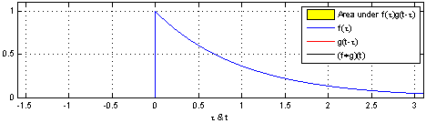
Note that in practice with CNNs, correlation is used instead of convolution, which is the same but without flipping the first function. There’s no need to “flip” a learned filter.
Key properties of convolutions
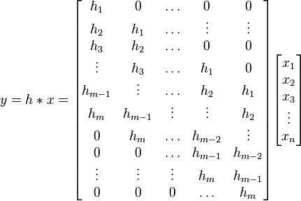
Convolution is a linear and shift-equivariant operator.
Linear means it can be represented simply as a matrix multiplication.
Shift-equivariance means that a shifted input will result in an output shifted by the same amount. Due to this property, the matrix representing a convolution has a special structure: it is always a Toeplitz matrix.
The shift-equivariance is an especially important property when dealing with images. Intuitively, an image of a cat is still an image of a cat, even if we shift it a few pixels to the right. This property ensures that a CNN layer applied to a shifted image will produce the same output features, but shifted. If our CNN can detect cats, it can will them regardless of their location in the image.
Hyperparameters & dimensions
What determines the output shape of a convolutional layer? Output shapes are often a source of confusion in practice, but they’re actually determined by a few simple things.
Let’s assume an input volume of shape
- Number of kernels,
. - Spatial extent (size) of each kernel,
. - Stride
: spatial distance between consecutive applications of a kernel. - Padding
: Number of “pixels” to zero-pad around each input feature map. - Dilation
: Spacing between kernel elements when applying to input.
I find the following animations (from this repo) are very helpful for visualizing the effect of these parameters. Below are a few parameter settings. Note that blue maps are inputs, green maps are outputs, and the shaded area is the kernel with
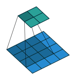 | 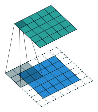 |  | 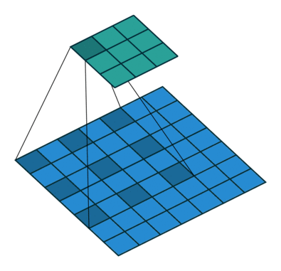 |
We can see that:
- The first option (left) produces an output smaller than the input. Without padding, there are only four locations the filter can be placed in, producing a
output. - The second option is like the first but with added padding of
. This leads to identical sizes of input and output feature maps because now the filter can be centered on each of the input pixels. - The third option demonstrates strides with
. A stride of means that the filter “jump” over two input pixels at a time. This again causes the output size to be smaller, even with padding. - The final option (right) demonstrates the effect of dilation. With
, the same number of kernel parameters are applied to a larger area of the input, by using non-contiguous input pixels. In terms of the output size, the effect is as if the kernel were larger, so the output is smaller.
So, given the hyperparameters,
-
Each convolution kernel will (usually) be a tensor of shape
. -
The output volume dimensions will be4:
-
The number of parameters in a convolutional layer will be:
For example, if we have an image of size
Pytorch example
Let’s see how the pytorch Conv2d layer works. Note that the “2d” in the name refers to the shape of the input feature maps, which, as we saw above, are indeed 2d in the case of images.
Let’s get some boilerplate out of the way. We’ll load the CIFAR10 image dataset so that we’ll have some data to work with, and then just print the shape of each image in the dataset.
import torchvision.transforms as tvtf

tf = tvtf.Compose([tvtf.ToTensor()])
ds_cifar10 = torchvision.datasets.CIFAR10(data_dir, download=True, train=True, transform=tf)
Files already downloaded and verified
# Load first CIFAR10 image
x0,y0 = ds_cifar10[0]

# add batch dimension
x0 = x0.unsqueeze(0)

# Note: channels come before spatial extent
print('x0 shape with batch dim:', x0.shape)
x0 shape with batch dim: torch.Size([1, 3, 32, 32])
Notice that we had to add an extra batch dimension because all pytorch layers expect to recieve a batch of elements. Also notice that the channel dimension comes before the height and width. This is the pytorch convension.
Let’s create a tiny utility function to count the number of parameters in an nn.Module.
def num_params(layer):
    return sum([p.numel() for p in layer.parameters()])
We can now create a conv layer with pytorch. Let’s count how many parameters it has, and compare it to what we expect based on the above.
import torch.nn as nn

# First conv layer: works on input image volume
conv1 = nn.Conv2d(in_channels=x0.shape[1], out_channels=10, padding=1, kernel_size=3, stride=1)

print(f'conv1: {num_params(conv1)} parameters')
conv1: 280 parameters
Which is indeed consistent with our calculation from above:
If we apply the layer to an input image, we can also see the output shape:
y1 = conv1(x0)
print(f'{"Input image shape:":25s}{x0.shape}')
print(f'{"After first conv layer:":25s}{y1.shape}')
Input image shape: torch.Size([1, 3, 32, 32])
After first conv layer: torch.Size([1, 10, 32, 32])
Let’s make our model deeper: a second conv layer will process the output volume of first layer. We need to make sure the number of output channels of the first later match the number of input channels of the second.
conv2 = nn.Conv2d(in_channels=10, out_channels=20, padding=0, kernel_size=6, stride=2)
print(f'conv2: {num_params(conv2)} parameters')

y2 = conv2(conv1(x0))
print(f'{"After second conv layer:":25s}{y2.shape}')
conv2: 7220 parameters
After second conv layer: torch.Size([1, 20, 14, 14])
Indeed, the new spatial extent matches our formula above:
Note
Notice how the width and height dimensions of the input image were never specified! all we had to provide was the inputs’ number of channels. More on the significance of that later.
Pooling layers
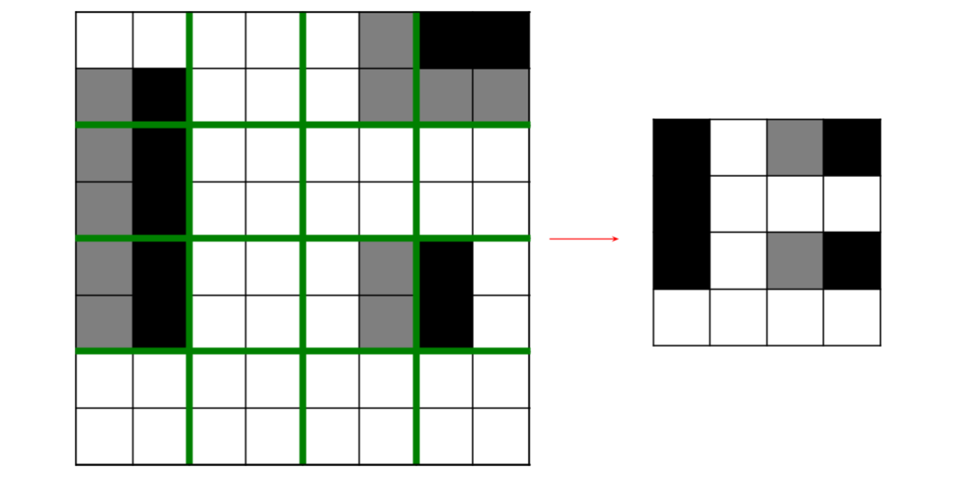
We saw how strides and dilation decrease the size of the input feature maps, producing smaller maps in the output. In addition to these parameters, another common way to reduce the size of feature maps between the convolutional layers is by adding pooling layers.
A pooling layer has the following hyperparameters (but no trainable parameters):
- Spatial extent (size) of each pooling kernel,
. - Stride
: spatial distance between consecutive applications. - Operation (e.g. max, average,
-norm)
Example: the image depicts a
Why pool feature maps after convolutions?
One reason is to more rapidly increase the receptive field of each layer. The receptive field of an element in a feature map is the set of elements in the input that can influence its value.
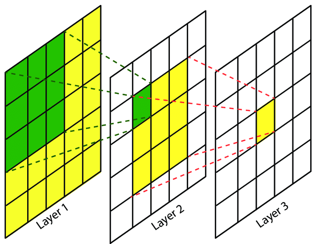
The receptive field size increases more rapidly if we add pooling, strides or dilation because by adding them, each feature map element becomes a function of more elements from the input feature map.
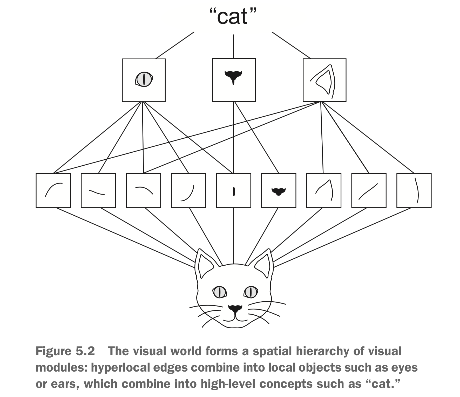
One intuition for why we want successive conv layers to be affected by increasingly larger parts of the input image, is that this allows us to learn a hierarchy of visual features. For example, when the filters in early layers learn to detect simple lines, the filters in later layers can learn to detect the presence of a combination of simple lines, forming a shape. Subsequence layers can learn to detect multiple shapes, which might allow e.g. the detection of a cat. This is all a bit hand-wavy, but there is indeed some evidence for this, of which we’ll see a bit below.
PyTorch example
A Pool2d layer works very similarly to the Conv2d we’ve seen above. We can create a factor-2 downsampling max-pooling layer as follows.
pool = nn.MaxPool2d(kernel_size=2, stride=2)

print(f'{"After second conv layer:":25s}{conv2(conv1(x0)).shape}')
print(f'{"After max-pool:":25s}{pool(conv2(conv1(x0))).shape}')
After second conv layer: torch.Size([1, 20, 14, 14])
After max-pool: torch.Size([1, 20, 7, 7])
Network Architecture
How do we actually use the convolutional layers we’ve been discussing to build a deep neural net, e.g. for image classification?
The basic architecture of a deep convolutional neural net is to repeat groups of conv-relu layers, optionally add pooling in between and end with a fully connected layer feeding into a softmax over the number of desired classes. Of course, there are many bells and whistles that can be added (such as residual connections, normalization layers, etc), but this is the most basic approach.
The image shows variants of the VGG architecture, one of the early successful deep CNNs.
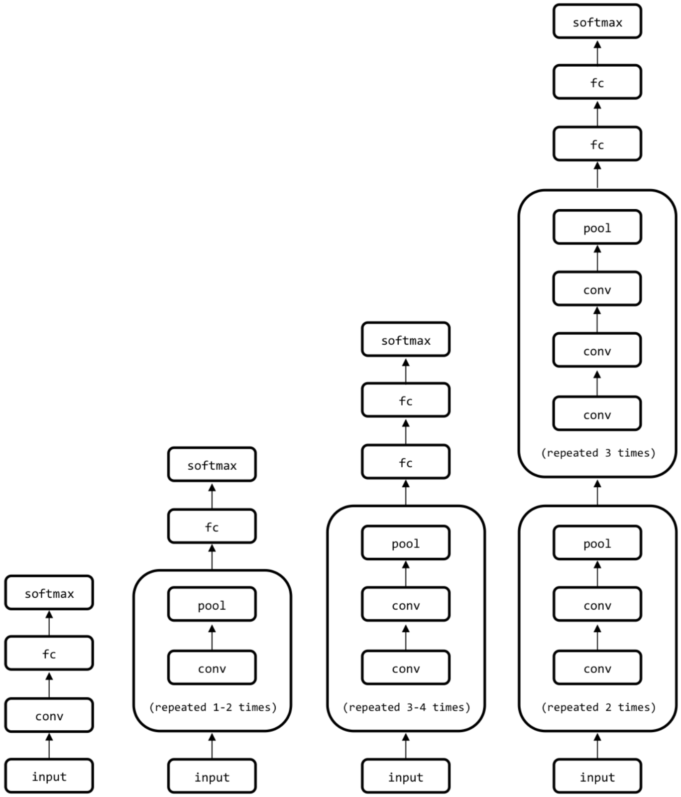
But why does such a scheme make sense, e.g. for image classification? Let’s break down what’s going on in the above image.
- All the conv blocks shown are actually conv-relu (or some other nonlinearity).
- The repeating conv-conv-…-pool blocks can be seen as learned non-linear feature extractors: they learn to detect specific features in an image (e.g. lines at different orientations).
- The pooling controls the receptive field increase, so that more high-level features can be generated by each conv group (e.g. shapes composed of multiple simple lines).
- The fully-connected layer and softmax at the end is just an MLP that uses the features extracted by the conv layers for multi-class classification (see also my previous post).
- Training this end-to-end means we train the classifier together with the features extractors!
There are many other things to consider as part of the architecture:
- Size of convolutional kernels
- Number of consecutive convolutions
- Use of batch normalization to speed up convergence
- Dropout for improved generalization
- Not using fully connected layers at all (we’ll see below)
- Skip connections (we’ll see below)
All of these could be hyperparameters to cross-validate over!
Many different network architectures exist, made famous mainly by repeated improvements on the ImageNet classification challenge since 2012.
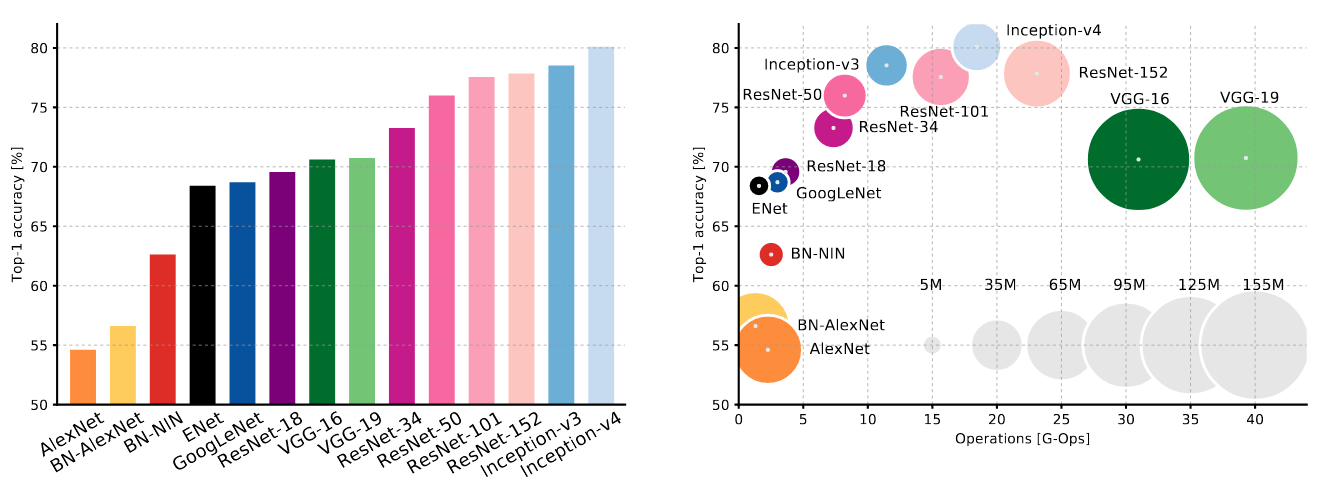
Some notable ImageNet-winning architectures include:
- AlexNet, 5 layers (2012): Based on LeNet, deeper, with ReLU, trained with GPUs
- Inception/GoogLeNet, 22 layers (2014): Multiple (small) kernel sizes at same depth
- ResNet, 152 (!) layers (2015): Skip connections
What kinds of filters are deep CNNs learning?
CNNs capture hierarchical features, with deeper layers capturing higher-level, class-specific features (Zeiler & Fergus, 2013).
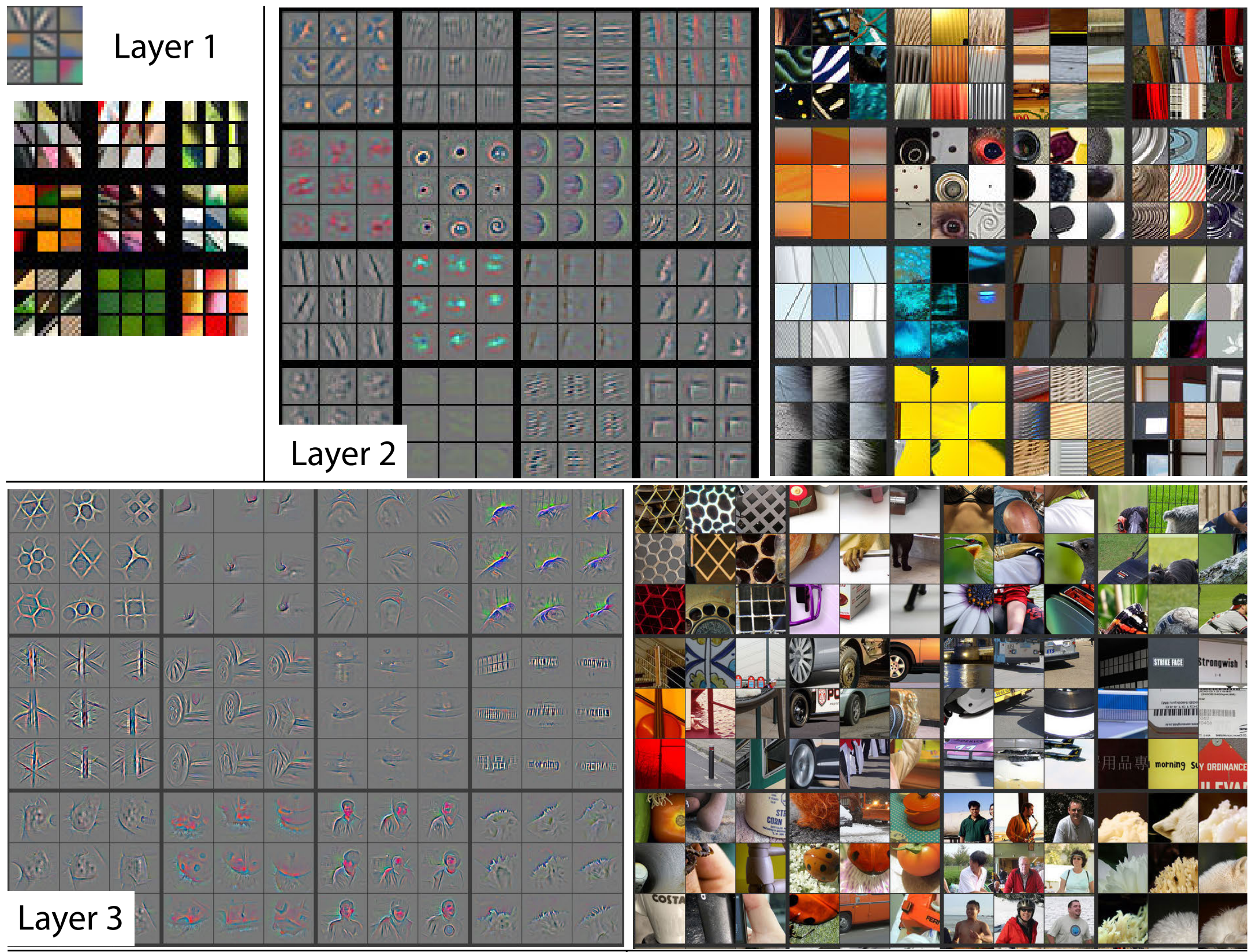
This visualization shows patterns which maximally activate kernels at various layers of a conv net, and the corresponding learned kernels (with false colors since they have more than three channels).
We can see how the layer 1 kernels look either like simple lines or color textures. Layer 2 kernels are already more complex, responding to some more compound shapes and complex textures. In layer 3, the filters learned to detect real-world objects such as car wheels and human faces.
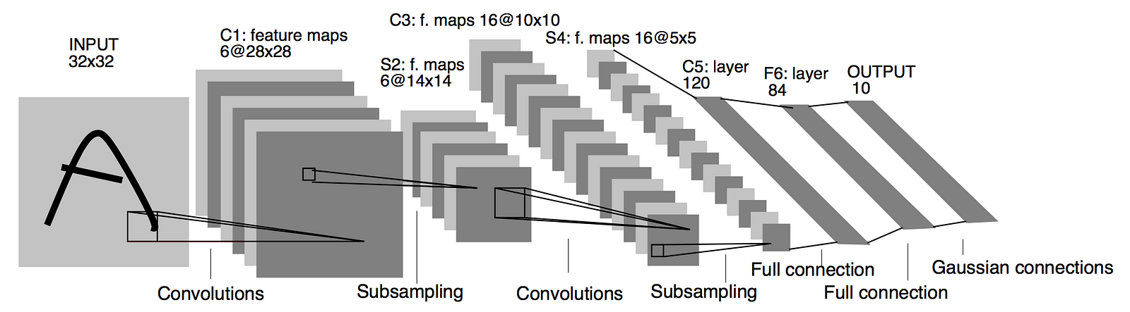
PyTorch network architecture example
As the simplest-possible example of a deep convolutional network, let’s implement LeNet, arguably the first successful CNN model for MNIST (LeCun, 1998). We’ll implement the architecture using built-in pytorch layers, according to the following diagram:
class LeNet(nn.Module):

    def __init__(self, in_channels=3):
        super().__init__()

        self.feature_extractor = nn.Sequential(
            nn.Conv2d(in_channels, out_channels=6, kernel_size=5),
            nn.ReLU(),
            nn.MaxPool2d(2),
            nn.Conv2d(in_channels=6, out_channels=16, kernel_size=5),
            nn.ReLU(),
            nn.MaxPool2d(2),
        )

        self.classifier = nn.Sequential(
            nn.Linear(16*5*5, 120), # Total number of features
            nn.ReLU(),
            nn.Linear(120, 84), # (N, 120) -> (N, 84)
            nn.ReLU(),
            nn.Linear(84, 10)   # (N, 84)  -> (N, 10)
        )

    def forward(self, x):
        # Extract conv features
        features = self.feature_extractor(x)
        # Flatten the features and feed to the classifier
        features = features.view(features.size(0), -1)
        class_scores = self.classifier(features)
        return class_scores
net = LeNet()
print(net)LeNet(
(feature_extractor): Sequential(
(0): Conv2d(3, 6, kernel_size=(5, 5), stride=(1, 1))
(1): ReLU()
(2): MaxPool2d(kernel_size=2, stride=2, padding=0, dilation=1, ceil_mode=False)
(3): Conv2d(6, 16, kernel_size=(5, 5), stride=(1, 1))
(4): ReLU()
(5): MaxPool2d(kernel_size=2, stride=2, padding=0, dilation=1, ceil_mode=False)
)
(classifier): Sequential(
(0): Linear(in_features=400, out_features=120, bias=True)
(1): ReLU()
(2): Linear(in_features=120, out_features=84, bias=True)
(3): ReLU()
(4): Linear(in_features=84, out_features=10, bias=True)
)
)
Note that there’s no softmax at the output here, we just return the raw class scores instead. Let’s make sure that the model works:
# Test forward pass
print('x0 shape=', x0.shape, end='\n\n')
print('LeNet(x0)=', net(x0), end='\n\n')
print('shape=', net(x0).shape)
x0 shape= torch.Size([1, 3, 32, 32])
LeNet(x0)= tensor([[ 0.0971, 0.0664, -0.0160, -0.1027, -0.1262, -0.0547, -0.0222, -0.0125,
0.0636, -0.0918]], grad_fn=<AddmmBackward>)
shape= torch.Size([1, 10])
Fully-convolutional Networks
Interestingly, we never actually specified the input image size when implementing LeNet in the previous example.
But does this mean we can use the network on images of any size?
No, because of the fully-connected layers at the end. Notice how we actually needed to know and hard-code the number of features in the input of the classifier (
Here, let’s try to present a larger image to this model:
large_image = torch.randn(1,3,32*2,32*2)
try:
    net(large_image)
except RuntimeError as e:
    print(e, file=sys.stderr)
size mismatch, m1: [1 x 2704], m2: [400 x 120] at /tmp/pip-req-build-q71pbt2d/aten/src/TH/generic/THTensorMath.cpp:41
How could we replace the FC layers at the end with something equivalent that requires no knowledge of the input image size? With more convolutions, of course!
To see how, let’s consider what would we be the result of a convolutional layer with
-
Kernels of size
, i.e. the full spatial extent of the input. Such a kernel can only “fit” once into the input volume, so the output would be just one single value. If we have K such kernels in our conv layer, we would get an output shape of . -
Kernels of size
. Such kernels can fit times into the input volume. The output will have the same shape as the input. Moreover, with convolutions, the each output element is only a function of the inputs at the same location. 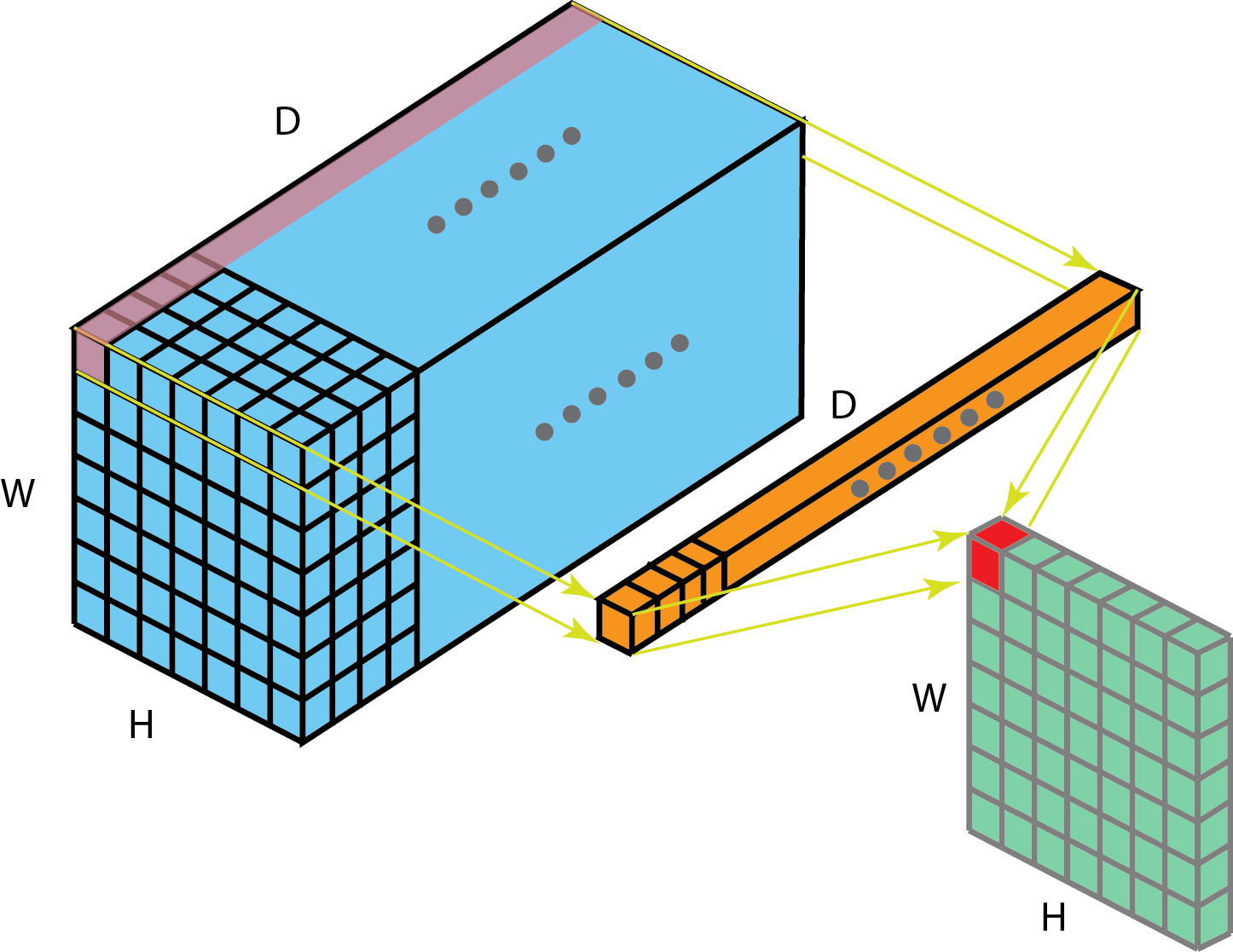
Now recall that in the classifier part in our LeNet projects the
Based on this, we can now create a fully-convolutional LeNet:
class LeNetFullyConv(LeNet):
    def __init__(self):
        super().__init__()
        # Remember: the last feature map volume has shape (16,5,5) for the original image size
        # Replace the base's classifier with 5x5 then 1x1 convolutions
        self.classifier = nn.Sequential(
            nn.Conv2d(in_channels=16, out_channels=120, kernel_size=5), # no padding or strides!
            nn.ReLU(),
            nn.Conv2d(in_channels=120, out_channels=84, kernel_size=1), # 1x1 conv
            nn.ReLU(),
            nn.Conv2d(in_channels=84, out_channels=10, kernel_size=1),  # 1x1 conv
        )

    def forward(self, x):
        # Using feature extractor block from the base model
        features = self.feature_extractor(x)
        # Note: no need to reshape the features now!
        class_scores = self.classifier(features)
        return class_scores
net_fully_conv = LeNetFullyConv()
print(net_fully_conv)LeNetFullyConv(
(feature_extractor): Sequential(
(0): Conv2d(3, 6, kernel_size=(5, 5), stride=(1, 1))
(1): ReLU()
(2): MaxPool2d(kernel_size=2, stride=2, padding=0, dilation=1, ceil_mode=False)
(3): Conv2d(6, 16, kernel_size=(5, 5), stride=(1, 1))
(4): ReLU()
(5): MaxPool2d(kernel_size=2, stride=2, padding=0, dilation=1, ceil_mode=False)
)
(classifier): Sequential(
(0): Conv2d(16, 120, kernel_size=(5, 5), stride=(1, 1))
(1): ReLU()
(2): Conv2d(120, 84, kernel_size=(1, 1), stride=(1, 1))
(3): ReLU()
(4): Conv2d(84, 10, kernel_size=(1, 1), stride=(1, 1))
)
)
Let’s forward the original-sized image and then also the larger image through the network and observe the output shapes:
print('regular image output shape:', net_fully_conv(x0).shape)
print('large   image output shape:', net_fully_conv(large_image).shape)
regular image output shape: torch.Size([1, 10, 1, 1])
large image output shape: torch.Size([1, 10, 9, 9])
For the regular sized image, the output is of shape
But the larger image has an output shape of
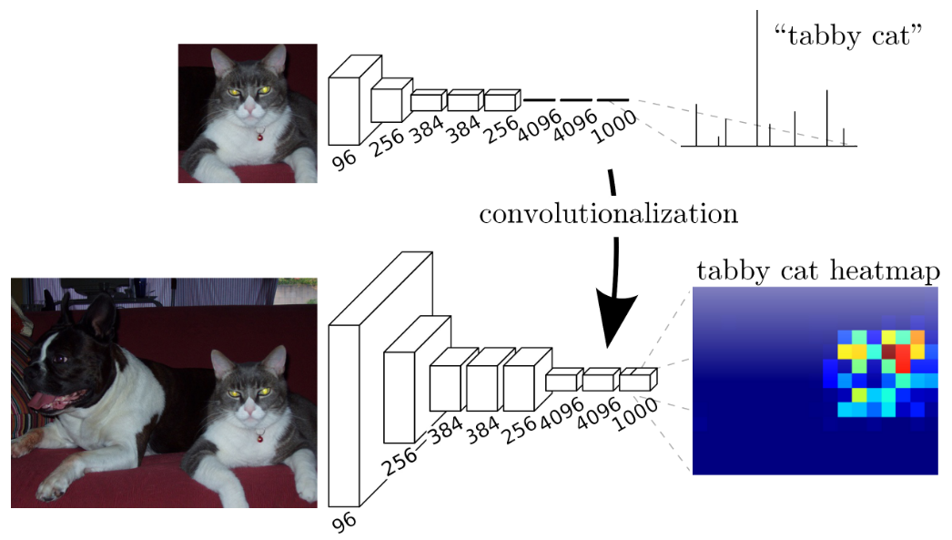
It’s now a spatial classification map! For a larger image, instead of getting 10 class scores, we get the class scores for multiple different locations on the original image. Here’s a visualization (from Long, 2015).
Residual Networks
For image-related tasks it seems that deeper is better: we could learn more complex, or high-level features.
How deep can we go? Should more depth always improve results?
In theory, adding an addition layer should provide at least the same accuracy as before because extra layers could always be just identity maps.
In practice, simply adding layers actually hurts performance. When adding depth, optimization issues arise, thereby making it harder to train the model to a well-performing parametrization.
One key issue with added depth is vanishing gradients, where the gradient of the loss w.r.t to parameters becomes tiny for the early parameters (which are “far” from the loss). This happens due to the chain rule, which creating a product with many terms for early parameters. For example, in a simple feed-forward network with weight tensors
this product becomes longer the deeper the network. If some of the terms are small, the product may become tiny. It then becomes effectively impossible to optimize some of these parameters with gradient descent, where the update in parameter values is proportional to the gradient.
The figure below demonstrates this (from He et al., 2015).
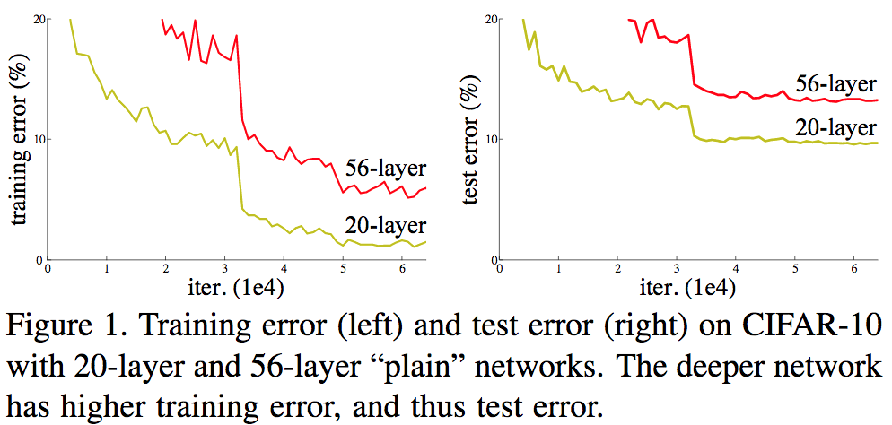
I.e., even if the same solution (or better) exists when the model is deeper, SGD-based optimization can’t find it. The optimization error increases with depth.
Residual networks, or ResNets, attempt to address these issues by building a network architecture composed of convolutional blocks with added shortcut-connections:
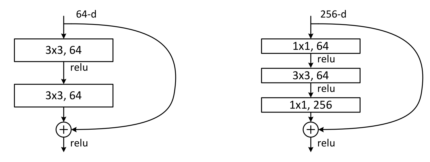
The idea is that the output of a residual block takes the form
Note that this requires that
In the diagram, the left side depicts a regular residual block, while the right side is called a bottleneck block. Bottleneck blocks reduce computational cost and the number of parameters by sandwiching a standard
Why do these shortcut-connections help?
The shortcuts create two key advantages:
- Allow gradients to “flow” freely backwards. The gradient of the loss with respect to a parameter tensor is the sum of the main feed-forward path (which may vanish) and the shortcut path (which is much less likely to vanish).
- Each block only learns the “residual mapping”, i.e. some delta from the identity map. Effectively, every block is now identity by default, and training only needs to learn to modify the identity map slightly.
Skip connections are so effective that virtually all modern CNNs utilize them in some way.
Conclusions
CNNs offer a robust solution to the challenges posed by fully-connected architectures for high-dimensional inputs like images. They exploit local connectivity and parameter sharing, not only to reduce the number of parameters, but also because the translation equivariant local filtering they perform inherently make sense for image data. The success of CNNs lies mainly in their ability to learn progressively abstract representations, tuned to the specific dataset and task at hand (e.g. classification).
Footnotes
-
The number of parameters in a convolutional layer does depend on one dimension of its input: the number of channels. In almost all images, this is 3. But inside a CNN, the internal convolutional layers produce input “images” with many channels for the next layer. ↩
-
Here we’re focused on images for simplicity, but actually not all CNNs have 2d features. 1d CNNs are also very common for signal processing applications, and 3d features are used e.g. for video. ↩
-
In this context, regular “parameters” are those that we train, while “hyperparameters” are those that we need to choose up-front, i.e. before training the model. ↩
-
For the full details, you’ll need to visit the relevant pytorch docs. ↩