Introduction
Logistic regression (LR) is a fundamental algorithm in machine learning and statistics. Despite its name, this is actually a classification model, where we’re trying to categorize data into two or more groups given some input features. Due to its simplicity, LR is widely used in many applications, especially for binary classification such as detecting whether an email is spam or not.
This post is a hands-on tutorial. We will build logistic regression from scratch, focusing on both the theory and implementation. Along the way, we will derive the logistic regression model based on maximum likelihood estimation.
We’ll implement the approach from scratch twice: first using NumPy to understand the underlying mechanics, and then using PyTorch to also leverage automatic differentiation. We’ll also extend the binary logistic regression model to handle multiclass problems using the softmax function.
This post should help you will understand the mathematical foundations of logistic regression, how it models probabilities for classification, and the steps involved in implementing it from scratch using NumPy and PyTorch. You will also explore its strengths and limitations in practical applications. See also my previous post for a broader intro about supervised learning and maximum likelihood estimation (which will be relevant here).
References
This post is based on materials created by me for the CS236781 Deep Learning course at the Technion between Winter 2019 and Spring 2022. To re-use, please provide attribution and link to this page.
Binary Logistic Regression
Given inputs
where
This function maps the real line onto
Notice how the LR model is actually a linear regression model wrapped in a sigmoid, to squash the output into the desired range. From a probabilistic perspective, we’re modeling the conditional probability to observe
Let’s take a look at the logistic function itself:
def logistic(z):
    return 1 / (1 + np.exp(-z))

x = np.arange(-5, 5, .01)
y_hat = logistic(x)

plt.plot(x, y_hat, label='$\sigma(z)$')
plt.grid(True); plt.xlabel('z'); plt.legend(); plt.title('The logistic function');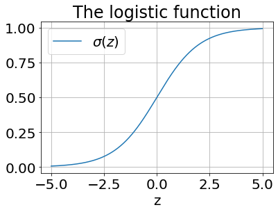
To fit the model, we’ll minimize the negative log-likelihood (equivalent to maximizing likelihood, i.e. MLE) of the parameters
We can then define our loss
The resulting pointwise loss is also known as (binary) cross-entropy:
The “cross” here is between the distribution of the samples
In this case, there’s no closed form solution, so we’ll need to train the model using some optimization scheme. Since this loss is convex, the gradient-based approach should lead us to the global optimum.
We can plot this loss function, to convince ourselves of its convexity.
loss_y0 = -np.log(1-y_hat)
loss_y1 = -np.log(y_hat)
plt.plot(y_hat, loss_y0, label='$\ell(y=0,\hat{y})$')
plt.plot(y_hat, loss_y1, label='$\ell(y=1,\hat{y})$')
plt.grid(True); plt.xlabel('$\hat{y}$'); plt.legend(); plt.title('Cross entropy loss');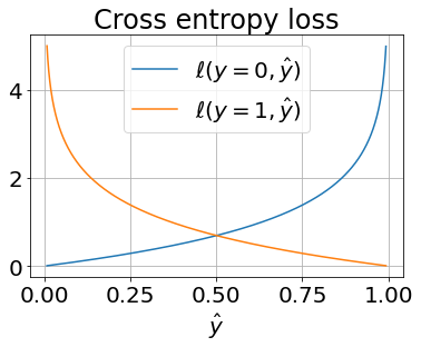
Next, to apply gradient descent, we’ll need to know the gradient of the loss w.r.t. the parameters
First, we apply the chain-rule
where
So we have found that for the cross entropy loss with binary logistic regression, the gradient is
Part 1: Binary Logistic Regression with numpy
As a warm-up, we’ll start by implementing this algorithm and training it from scratch using just numpy (and a toy dataset from sklearn).
This is a classic and elementary example of implementing and training a machine learning algorithm. By first using only numpy, we get to see the barebone details without the help of any fancy machine-learning library.
Dataset
The scikit-learn library comes with a few toy datasets that are fun to quickly train small models on.
As an example, we’ll load the Wisconsin-breast cancer database:
- 569 samples of cancer patients
- 30 features: various properties of tumor cells extracted from images
- 2 classes: Tumor is either Benign or Malignant
We’ll apply the basic machine learning approach we saw above: binary logistic regression.
import sklearn.datasets

ds_cancer = sklearn.datasets.load_breast_cancer()
feature_names = ds_cancer.feature_names
target_names = ds_cancer.target_names
n_features = len(feature_names)

print(f'{n_features=}')
print(f'feature names: {feature_names}')
print(f'target  names: {target_names}')
n_features=30
feature names: ['mean radius' 'mean texture' 'mean perimeter' 'mean area'
'mean smoothness' 'mean compactness' 'mean concavity'
'mean concave points' 'mean symmetry' 'mean fractal dimension'
'radius error' 'texture error' 'perimeter error' 'area error'
'smoothness error' 'compactness error' 'concavity error'
'concave points error' 'symmetry error' 'fractal dimension error'
'worst radius' 'worst texture' 'worst perimeter' 'worst area'
'worst smoothness' 'worst compactness' 'worst concavity'
'worst concave points' 'worst symmetry' 'worst fractal dimension']
target names: ['malignant' 'benign']
X, y = ds_cancer.data, ds_cancer.target
n_samples = len(y)

print(f'X: {X.shape}')
print(f'y: {y.shape}')
X: (569, 30)
y: (569,)
First we need to handle the data: loading, splitting and processing it. We start by loading it into a pandas dataframe and show some samples.
y_names = np.full_like(y, target_names[0].upper(), dtype=target_names.dtype)
y_names[y==1] = target_names[1].upper()

df_cancer = pd.DataFrame(data=X, columns=ds_cancer.feature_names)
df_cancer = df_cancer.assign(CLASS=y_names)
df_cancer.iloc[100:110, 0::3]| mean radius | mean area | mean concavity | mean fractal dimension | perimeter error | compactness error | symmetry error | worst texture | worst smoothness | worst concave points | CLASS | |
|---|---|---|---|---|---|---|---|---|---|---|---|
| 100 | 13.610 | 582.7 | 0.08625 | 0.05871 | 2.8610 | 0.014880 | 0.01465 | 35.27 | 0.1265 | 0.11840 | MALIGNANT |
| 101 | 6.981 | 143.5 | 0.00000 | 0.07818 | 1.5530 | 0.010840 | 0.02659 | 19.54 | 0.1584 | 0.00000 | BENIGN |
| 102 | 12.180 | 458.7 | 0.02383 | 0.05677 | 1.1830 | 0.006098 | 0.01447 | 32.84 | 0.1123 | 0.07431 | BENIGN |
| 103 | 9.876 | 298.3 | 0.06154 | 0.06322 | 1.5280 | 0.021960 | 0.01609 | 26.83 | 0.1559 | 0.09749 | BENIGN |
| 104 | 10.490 | 336.1 | 0.02995 | 0.06481 | 2.3020 | 0.022190 | 0.02710 | 23.31 | 0.1219 | 0.03203 | BENIGN |
| 105 | 13.110 | 530.2 | 0.20710 | 0.07692 | 2.4100 | 0.029120 | 0.01547 | 22.40 | 0.1862 | 0.19860 | MALIGNANT |
| 106 | 11.640 | 412.5 | 0.07070 | 0.06520 | 2.1550 | 0.023100 | 0.01565 | 29.26 | 0.1688 | 0.12180 | BENIGN |
| 107 | 12.360 | 466.7 | 0.02643 | 0.06066 | 0.8484 | 0.010470 | 0.01251 | 27.49 | 0.1184 | 0.08442 | BENIGN |
| 108 | 22.270 | 1509.0 | 0.42640 | 0.07039 | 10.0500 | 0.086680 | 0.03112 | 28.01 | 0.1701 | 0.29100 | MALIGNANT |
| 109 | 11.340 | 396.5 | 0.05133 | 0.06529 | 1.5970 | 0.015570 | 0.01568 | 29.15 | 0.1699 | 0.08278 | BENIGN |
We’ll produce a basic split into train and test sets.
from sklearn.model_selection import train_test_split

X_train, X_test, y_train, y_test = train_test_split(X, y, test_size=0.3, random_state=42, stratify=y)

print(f'train: X={X_train.shape} y={y_train.shape}')
print(f'test : X={X_test.shape} y={y_test.shape}')
train: X=(398, 30) y=(398,)
test : X=(171, 30) y=(171,)
And finally, we’ll standardize the features.
# Note: each feature is standardized individually:
mu_X = np.mean(X_train, axis=0) # (N, D) -> (D,)
sigma_X = np.std(X_train, axis=0)

# Note: Broadcasting (N, D) with (D,) -> (N, D)
X_train_sc = (X_train - mu_X) / sigma_X

# Note: Test set must be transformed identically to training set
X_test_sc = (X_test - mu_X) / sigma_X

print(f'{mu_X.shape=}, {sigma_X.shape=}')
mu_X.shape=(30,), sigma_X.shape=(30,)
Model Implementation
We can now implement the model based on the above definitions. To make it cleaner, we’ll implement it as a class with an API that conforms to the sklearn models. See sklearn’s LogisticRegression class.
class BinaryLogisticRegression(object):
    def __init__(self, n_iter=100, learn_rate=0.1):
        self.n_iter = n_iter
        self.learn_rate = learn_rate
        self._w = None

    def _add_bias(self, X: np.ndarray):
        # Add a bias term column
        ones_col = np.ones((X.shape[0], 1))
        return np.hstack([ones_col, X])

    def predict_proba(self, X: np.ndarray, add_bias=True):
        X = self._add_bias(X) if add_bias else X

        # Apply logistic model
        z = np.dot(X, self.weights) # (N, D) * (D,)
        return logistic(z) # shape (N,)

    def predict(self, X: np.ndarray):
        proba = self.predict_proba(X)

        # Apply naive threshold of .5
        return np.array(proba > .5, dtype=np.int)

    def fit(self, X: np.ndarray, y: np.ndarray):
        n, d = X.shape # X is (N, D), y is (N,)

        # Initialize weights
        self._w = np.random.randn(d + 1) * 0.1

        Xb = self._add_bias(X)

        # Training loop
        self._losses = []
        for i in range(self.n_iter):
            # Predicted probabilities
            y_hat = self.predict_proba(Xb, add_bias=False)

            # Pointwise loss
            loss = -y.dot(np.log(y_hat)) - ((1 - y).dot(np.log(1 - y_hat)))

            # See gradient derivation above
            loss_grad = 1/n * Xb.T.dot(y_hat - y)  # dl/dw: (D+1, N) * (N,)

            # Optimization step
            self._w += -self.learn_rate * loss_grad
            self._losses.append(loss)

        return self

    @property
    def weights(self):
        if self._w is None:
            raise ValueError("Model is not fitted")
        return self._w
Notice that we implemented the training loop in the fit() method. We can now use it to train the model and show a basic loss curve.
lr_model = BinaryLogisticRegression(n_iter=500, learn_rate=0.01)
lr_model.fit(X_train_sc, y_train)

plt.plot(lr_model._losses, label='$L_{\mathcal{S}}$');
plt.xlabel('training iteration');
plt.legend(); plt.grid(True);
plt.title('Train loss');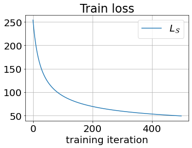
On this toy dataset, our performance is quite good. This is just a useful sanity check that we implemented the model correctly.
y_train_pred = lr_model.predict(X_train_sc)
train_acc = np.mean(y_train_pred == y_train)
print(f'train set accuracy: {train_acc*100:.2f}%')

y_test_pred = lr_model.predict(X_test_sc)
test_acc = np.mean(y_test_pred == y_test)
print(f'test set accuracy: {test_acc*100:.2f}%')
train set accuracy: 96.73%
test set accuracy: 95.91%
Part 2: Multiclass Logistic Regression with pytorch
What if we actually have
A naïve approach: train
One major drawback of this approach is that it doesn’t model a probability distribution over the possible classes,
Let’s introduce a better approach, which extends logistic regression to the multi-class setting.
The softmax function
Softmax is a function which generates a discrete probability distribution for our
note that this is a vector-valued and multivariate function. The exponent in the enumerator operates elementwise on its vector input. The result of softmax is a vector with elements in
The multiclass model
Our model can now be defined as
where,
is a vector of class probabilities. is a sample. is a matrix representing the per-class weights. is a per-class bias vector of length .
Probabilistic interpretation:
While not very powerful on its own, this type of model is commonly found at the end of deep neural networks performing classification tasks.
The target variable is usually specified as an index of the correct class. However, to train this model, we need our labels to also be discrete probability distributions instead of simply a label.
We’ll transform our labels to a 1-hot encoded vector corresponding to a singleton distribution (all mass is on a single class). For example, if
and this will be the target variable corresponding to
Cross-Entropy loss
After defining the 1-hot label vectors, the multiclass extension of the binary cross-entropy is straightforward:
Note that only the probability assigned to the correct class affects the loss because
Minimizing this cross entropy can be interpreted as trying to move the probability distribution of model predictions towards the singleton distribution of the appropriate class.
Dataset
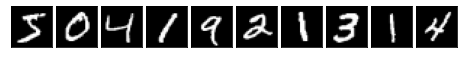
This time we’ll tackle an image classification task, the MNIST database of handwritten digits. These days, this is also considered a toy dataset, even though it was widely used in the past to benchmark classification algorithms.
import os
import torch
import torch.autograd
import torch.utils.data
import torchvision
import torchvision.transforms
import plot_utils

from torch import Tensor
We’ll load the data using standard pytorch datasets and data loaders. We’ll also need to define the transforms that should be applied to each image in the dataset before returning it.
tf_ds = torchvision.transforms.ToTensor()

batch_size = 64
data_root = os.path.expanduser("~/.pytorch-datasets")

# Training and test datasets
ds_train, ds_test = [
    torchvision.datasets.MNIST(root=data_root, download=True, train=train, transform=tf_ds)
    for train in [True, False]
]

# Data loaders
dl_train = torch.utils.data.DataLoader(ds_train, batch_size, shuffle=True)
dl_test = torch.utils.data.DataLoader(ds_test, batch_size=len(ds_test))

x0, y0 = ds_train[0]
n_features = torch.numel(x0)
n_classes = 10
Let’s see what the first few samples look like.
print(f'x0: {x0.shape}, y0: {y0}')
plot_utils.dataset_first_n(ds_train, 10, cmap='gray');
x0: torch.Size([1, 28, 28]), y0: 5
Note that when training, we’re actually working with batches of samples, as we’ll be using stochastic gradient descent (SGD). So each input image is actually a four-dimensional tensor:
x0, y0 = next(iter(dl_train))
x0.shape
torch.Size([64, 1, 28, 28])
Model Implementation
This time we’ll use pytorch tensors and its autograd functionality to implement our model. This means we won’t have to implement any gradient calculations!
First, let’s implement
def softmax(z: Tensor) -> Tensor:
    """
    softmax(z)= e^(z) / sum(e^z)
    :param z: A batch of C class scores per N samples, shape (N, C).
    :returns: softmax per sample, of shape (N, C).
    """

    # normalization trick to prevent numerical instability:
    # shift so that the highest class score (per sample) is 0
    zmax, _ = torch.max(z, dim=1, keepdim=True)
    z = z - zmax # note broadcasting: (N,C) - (N,1)

    exp_z = torch.exp(z) # (N, C)
    sum_exp = torch.sum(exp_z, dim=1, keepdim=True) # (N, 1)
    return exp_z / sum_exp # probabilities, (N,C)
Let’s test our softmax and calculate its derivative with autograd.
z = torch.randn(size=(4,3), requires_grad=True)
y = softmax(z)
y
tensor([[0.1167, 0.7073, 0.1760],
[0.0702, 0.7838, 0.1460],
[0.0755, 0.4197, 0.5048],
[0.0205, 0.1090, 0.8704]], grad_fn=<DivBackward0>)
To calculate gradient autograd.grad() as follows:
y = softmax(z)
L = torch.sum(y) # scalar function of z

torch.autograd.grad(L, z)
(tensor([[0., 0., 0.],
[0., 0., 0.],
[0., 0., 0.],
[0., 0., 0.]]),)
Instead of calling autograd.grad() directly with specific input tensors, pytorch provides us with a way to calculate the derivative of a tensor w.r.t. all the tensors which are leaves in its computation graph (only
This can be done by calling .backward() on a scalar tensor. As a result, the .grad property of leaf tensors will be populated with the gradient:
# Example with two leaves in the computaion graph
z1 = torch.randn(size=(4,3), requires_grad=True)
z2 = torch.randn(size=(1,3), requires_grad=True)
z = z1 - z2

y = softmax(z)
L = torch.sum(y) # scalar function of z
L.backward()     # Calculate derivative w.r.t. all leaves

z1.grad, z2.grad # The leaves z1, z2 will have their .grad populated
(tensor([[0., 0., 0.],
[0., 0., 0.],
[0., 0., 0.],
[0., 0., 0.]]),
tensor([[0., 0., 0.]]))
We can visualize the resulting computation graph, and ensure that it corresponds to how we implemented our model.
import torchviz
torchviz.make_dot(L, params=dict(z1=z1, z2=z2))
The next ingredient of the solution is the cross-entropy loss function.
def cross_entropy_loss(y: Tensor, y_hat: Tensor, eps=1e-6):
    """
    :param y:  Onehot-encoded ground-truth labels, shape (N, C)
    :param y_hat: A batch of probabilities, shape (N,C)
    :returns: Cross entropy between y and y_hat.
    """
    return torch.sum( - y * torch.log(y_hat + eps) )
Recall that we need to encode our ground-truth labels as one-hot vectors to apply the multiclass cross-entropy. We can implement this functionality as a small utility function:
def onehot(y: Tensor, n_classes: int) -> Tensor:
    """
    Encodes y of shape (N,) containing class labels in the range [0,C-1] as one-hot of shape (N,C).
    """
    y = y.reshape(-1, 1) # Reshape y to (N,1)
    zeros = torch.zeros(size=(len(y), n_classes), dtype=torch.float32) # (N,C)
    ones = torch.ones_like(y, dtype=torch.float32)

    # scatter: put items from 'src' into 'dest' at indices correspondnig to 'index' along 'dim'
    y_onehot = torch.scatter(zeros, dim=1, index=y, src=ones)

    return y_onehot # result has shape (N, C)
If we apply it to a vector of class labels, we can see that each label gets expanded to a tensor, where only the corresponding index is set to 1.
onehot(torch.tensor([1, 3, 5, 0]), n_classes=10)tensor([[0., 1., 0., 0., 0., 0., 0., 0., 0., 0.],
[0., 0., 0., 1., 0., 0., 0., 0., 0., 0.],
[0., 0., 0., 0., 0., 1., 0., 0., 0., 0.],
[1., 0., 0., 0., 0., 0., 0., 0., 0., 0.]])
Our model itself will just be a class which holds the parameters tensors forward() function. Note also that this implementation does not use pytorch’s Module class. We’ll instead keep it as simple as possible, and only usepytroch for its tensors and automatic differentiation.
class MCLogisticRegression(object):
    def __init__(self, n_features: int, n_classes: int):
        # Define our parameter tensors: notice that now W and b are separate
        # Specify we want to track their gradients with autograd
        self.W = torch.randn(n_features, n_classes, requires_grad=True)
        self.b = torch.randn(n_classes, requires_grad=True)
        self.params = [self.W, self.b]

    def __call__(self, *args):
        return self.forward(*args)

    def forward(self, X: Tensor):
        """
        :param X: A batch of samples, (N, D)
        :return: A batch of class probabilities, (N, C)
        """
        # X is (N, D), W is (D, C), b is (C,)
        z = torch.mm(X, self.W) + self.b
        y_hat = softmax(z)
        return y_hat # (N, C)
Let’s try out the model and loss on the first batch. Note that we naïvely treat each pixel as a separate feature. We’ll learn how to properly work with images in a future post.
model = MCLogisticRegression(n_features, n_classes)

# Flatten images and convert labels to onehot
x0_flat = x0.reshape(-1, n_features)
y0_onehot =  onehot(y0, n_classes)

print(f'x0_flat: {x0_flat.shape}')
print(f'y0_onehot: {y0_onehot.shape}\n')
x0_flat: torch.Size([64, 784])
y0_onehot: torch.Size([64, 10])
We can also run a forward pass and compute loss:
y0_hat = model(x0_flat)
loss = cross_entropy_loss(y0_onehot, y0_hat)
print('loss = ', loss)

# Backward pass to populate .grad on leaf nodes
loss.backward()
loss = tensor(611.5060, grad_fn=<SumBackward0>)
Since we specified require_grad=True for our model parameters, every operation performed on these tensors is recorded, and a computation graph can be built, which included the model and loss calculation.
Notice that the leaves in this graph are our parameters
import torchviz
torchviz.make_dot(loss, params=dict(W=model.W, b=model.b))
This graph is what allows efficient implementation of the back-propagation algorithm, which you’ll learn about in the next lecture.
By calling .backward() from the final loss tensor, pytorch automatically populated the .grad property of all leaves in this graph, without us having to explicitly specify them (W and b).
Training
The optimization will be as before, but now we’ll take the gradients from the grad property of our parameter tensors. Therefore, the optimizer needs access only to the parameter tensors from the model. In fact, pytorch’s Optimizer classes work in the same way.
As before, we’ll implement this from scratch using only pytorch tensors and no other build-in features.
from typing import Sequence

class SGDOptimizer:
    """
    A simple gradient descent optimizer.
    """
    def __init__(self, params: Sequence[Tensor], learn_rate: float):
        self._params = params
        self._learn_rate = learn_rate

    def step(self):
        """
        Updates parameters in-place based on their gradients.
        """
        with torch.autograd.no_grad(): # Don't track this operation
            for param in self._params:
                if param.grad is not None:
                    param -= self._learn_rate * param.grad

    def zero_grad(self):
        """
        Zeros the parameters' gradients if they exist.
        """
        for param in self._params:
            if param.grad is not None:
                param.grad.zero_()
Without training anything yet, we can calculate the prediction accuracy as a sanity check.
def evaluate_accuracy(dataloader, model, max_batches=None):
    n_correct = 0.
    n_total = 0.
    for i, (X, y) in enumerate(dataloader):
        X = X.reshape(-1, n_features) # flatten images into vectors

        # Forward pass
        with torch.autograd.no_grad():
            y_hat = model(X)

        predictions = torch.argmax(y_hat, dim=1)
        n_correct += torch.sum(predictions == y).type(torch.float32)
        n_total += X.shape[0]

        if max_batches and i+1 >= max_batches:
            break

    return (n_correct / n_total).item()

test_set_acc = evaluate_accuracy(dl_test, MCLogisticRegression(n_features, n_classes))
print(f'Test set accuracy pre-training: {test_set_acc*100:.2f}%')
Test set accuracy pre-training: 7.65%
We can see that without training, the models’ accuracy is roughly
The training loop
Training loops are a crucial part of any ML pipeline, where model parameters get updated iteratively.
When using pytorch, the training loop will generally contain the following steps:
- Each epoch:
- Split training data into batches
- For each batch
- Forward pass: Compute predictions and build computation graph
- Calculate loss
- Set existing gradients to zero
- Backward pass: Use back-propagation algorithm to calculate the gradients
- Optimization step: Use the gradients to update the parameters
- Evaluate accuracy on validation set
Notice that one pass over the entire training data is called an epoch.
Let’s define some sane training hyperparameters and instantiate the model.
epochs = 10
max_batches = 50  # limit batches so training is fast (just as a demo)
learn_rate = .005
num_samples = len(ds_train)

# Instantiate the model we'll train
model = MCLogisticRegression(n_features, n_classes)

# Instantiate the optimizer with model's parameters
optimizer = SGDOptimizer(model.params, learn_rate=learn_rate)
Now we can start training. Below is the implementation of the training loop based on what we outlined above.
# Epoch: traverse all samples
for e in range(epochs):
    cumulative_loss = 0

    # Loop over randdom batches of training data
    for i, (X, y) in enumerate(dl_train):

        X = X.reshape(-1, n_features)
        y_onehot = onehot(y, n_classes)

        # Forward pass: predictions and loss
        y_hat = model(X)
        loss = cross_entropy_loss(y_onehot, y_hat)

        # Clear previous gradients
        optimizer.zero_grad()

        # Backward pass: calculate gradients
        loss.backward()

        # Update model using the calculated gradients
        optimizer.step()

        cumulative_loss += loss.item()
        if i+1 > max_batches:
            break

    # Evaluation
    test_accuracy = evaluate_accuracy(dl_test, model, max_batches)
    train_accuracy = evaluate_accuracy(dl_train, model, max_batches)

    avg_loss = cumulative_loss/num_samples
    print(f"Epoch {e}. Avg Loss: {avg_loss:.3f}, Train Acc: {train_accuracy*100:.2f}, Test Acc: {test_accuracy*100:.2f}")
Epoch 0. Avg Loss: 0.352, Train Acc: 41.69, Test Acc: 43.67
Epoch 1. Avg Loss: 0.161, Train Acc: 63.34, Test Acc: 63.29
Epoch 2. Avg Loss: 0.099, Train Acc: 70.88, Test Acc: 71.77
Epoch 3. Avg Loss: 0.075, Train Acc: 74.84, Test Acc: 76.31
Epoch 4. Avg Loss: 0.064, Train Acc: 78.12, Test Acc: 78.12
Epoch 5. Avg Loss: 0.058, Train Acc: 79.03, Test Acc: 79.77
Epoch 6. Avg Loss: 0.053, Train Acc: 80.03, Test Acc: 81.39
Epoch 7. Avg Loss: 0.050, Train Acc: 80.84, Test Acc: 82.08
Epoch 8. Avg Loss: 0.051, Train Acc: 81.88, Test Acc: 83.58
Epoch 9. Avg Loss: 0.047, Train Acc: 83.00, Test Acc: 83.77
Final notes
This is a very naïve implementation, for example because
- We didn’t treat the images properly.
- We didn’t include any regularization.
We could’ve utilized several functions and classes that PyTorch provides, such as:
- Fully connected layer with model parameters
- Softmax
- SGD and many other optimizers
- Cross entropy loss
However, the purpose here was to show an (almost) from-scratch implementation using only tensors, to see what’s “under the hood” (more or less) of the PyTorch functions.