Building an MLP from scratch

Introduction

Multilayer perceptrons (MLPs) form the basis of deep learning. They are arguably the simplest “deep” models and are ubiquitous in many applications. Although more advanced architectures such as CNNs or Transformers are often employed to exploit the domain-specific structure of the data (e.g. in the case of images), the humble MLP can still be found in and around such architectures: up/down projecting features between various layers or towards the output.

In this hands-on tutorial, we will implement an MLP model from scratch. First, we’ll do it purely in numpy, including all the required derivations for gradient computation. Then, we’ll reimplement a more general version using PyTorch and familiarize ourselves with some basic PyTorch APIs such as modules, loss functions and optimizers.

References

This post is based on materials created by me for the CS236781 Deep Learning course at the Technion between Winter 2019 and Spring 2022. To re-use, please provide attribution and link to this page.

Some images in the post were taken and/or adapted from the following sources:

• Pattern Recognition and Machine Learning, C. M. Bishop, Springer, 2006
• Fundamentals of Deep Learning, Nikhil Buduma, O’Reilly 2017
• MartinThoma [CC0], via Wikimedia Commons: Perceptron Unit.svg
• https://sebastianraschka.com/Articles/2015_singlelayer_neurons.html
• https://towardsdatascience.com/a-conversation-about-deep-learning-9a915983107

Perceptrons and linear models

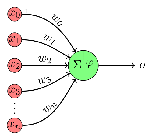
The following hypothesis class,

where is some nonlinear function, is known as the perceptron model. We can see that this type of model first applies an affine transform to its input, just like a linear regression model. The difference is the additional non-linear transformation applied at the end.

In a previous post we trained a logistic regression model by using the sigmoid function as our :

A significant limitation of logistic regression it’s only a linear classifier. In what sense is it linear though? Didn’t we just add a non-linear function at the end?

A function like is linear in the sense that output depends only on a linear combination of weights and inputs. Such a model will only be able to perfectly classify data if it’s linearly separable:

If we consider , then the decision boundary of the classifier is the set of all points where (usually zero). For a linear model, the decision boundaries are lines (or surfaces if ):

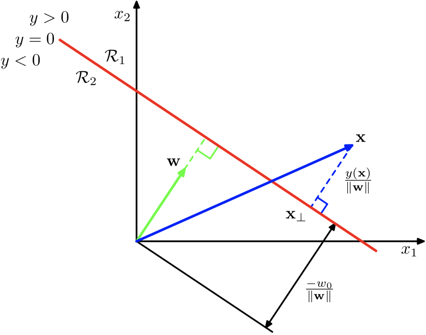
Note that in the diagram, . We can see that,

1. For any on the decision boundary, . This means that is orthogonal to every vector in the surface.
2. For any on the decision boundary, . Since is the length of the projection of onto , then the distance of the boundary from origin is given by .
3. For any point , is the signed perpendicular distance from the decision boundary.

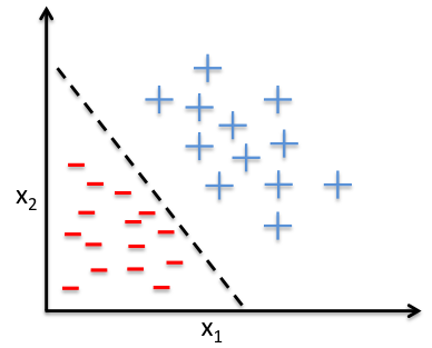
What if our data is not linearly separable? Can we still use e.g. logistic regression?

What if we first apply a fixed non-linear transformation to the data? Consider: For some , what does the following classifier do?

We still get a linear decision boundary, but it’s relative to the new features . Projecting this boundary back to , we can get nonlinear decision boundaries with respect to the original .

But how can we choose a nonlinear transformation?

The traditional machine learning approach would be to craft it painstakingly based on domain-knowledge. This is usually known as feature-engineering and was a crucial part of almost any machine-learning task, especially when complex or high-dimensional input data is required, like in computer vision.

But what if we want to learn to extract the features together with the classifier itself? That’s where deep learning comes in. And the simplest example is that we’ll see next.

Multilayer Perceptron (MLP)

Model

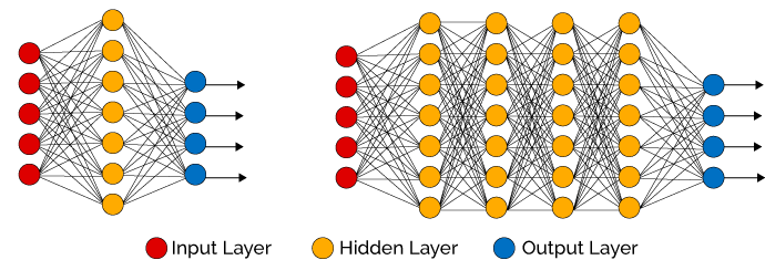
As its name suggests, an MLP is composed of layers, each layer with perceptron (“neuron”) units.

Each layer operates on the output of the previous layer () and calculates:

• Note that both input and output are vectors. We can think of the above equation as describing a layer of multiple perceptrons.
• We’ll henceforth refer to such layers as fully-connected or FC layers.
• The first layer accepts the input of the model, i.e. .
• The last layer, , is the output layer, so is the output of the model.
• The layers are called hidden layers.

The MLP can theoretically approximate any function, making it a very potent hypothesis class (recall approximation error).

Universal approximator theorem (informal)

Given enough parameters, an MLP with and any non-linear activation function, can approximate any continuous function up to any specified precision (Cybenko, 1989).

See here for a great intuitive explanation of the UAT.

Given an input sample , the computed function of an -layer MLP is:

I.e., this is a composition of functions. Assuming is differentiable, each of these functions is differentiable and so is their composition. The MLP model output is therefore fully differentiable w.r.t. parameters using the Chain Rule.

Notice that if we look only at the last layer, we can see that is just the linear model we started with. So, intuitively, we can think of as a set of learned non-linear features of the input! In other words, .

Since an MLP it has a non-linear dependency on its inputs, through a learned transformation, non-linear decision boundaries are possible.

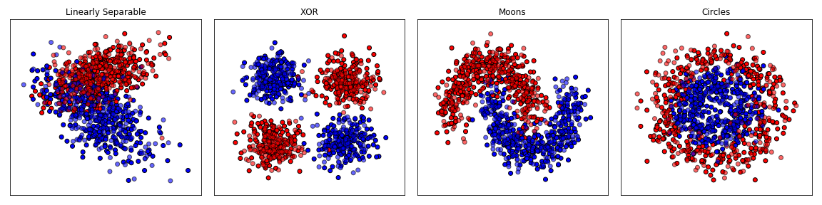
For example, here are the decision boundaries for three MLPs with 1, 2 and 4 hidden layers of 3 neurons each, and a single output feature for binary classification: 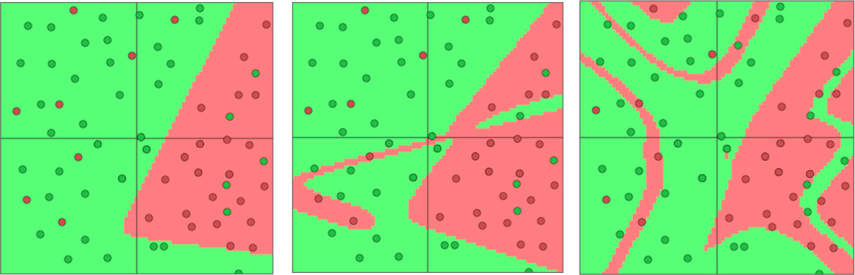In these examples, the input space has two features, from which three new features are learned, and the MLP produces it’s classification based on these three features.

Visualization of hand-crafted vs. MLP-learned features

A great visualization of the effect of features and MLP layers can be found at the tensorflow playground.

For example, using the circles dataset which has two input features, see what happens with:

• No hidden layers (classifier applied directly on input)
• One hidden layer, two neurons (same as input)
• One hiddlen layer, three neurons (additional learned feature)

Activation functions

An activation function is the non-linear elementwise function which operates on the affine part of the perceptron model. But why do we even need non-linearities in the first place? Isn’t the depth enough?

Without them, the MLP model would be equivalent to a single affine transform.

Common choices for the activation functions are:

• The logistic function, i.e. sigmoid:

• The hyperbolic tangent, which is a shifted and scaled sigmoid:

• The rectified linear unit (ReLU), which simply clamps negative values to zero:

  Note that ReLU is not strictly differentiable. However, sub-gradients exist. For the purpose of computing the gradients of our model, we can define the gradient of ReLU as,

We can plot some activation functions and their gradients to see what they look like.

# Activation functions
relu = lambda x: np.maximum(0, x)
sigmoid = lambda x: 1 / (1 + np.exp(-x))
tanh = lambda x: (np.exp(x)-np.exp(-x)) / (np.exp(x)+np.exp(-x))
 
# Their gradients
g_relu = lambda x: np.array(relu(x) > 0, dtype=np.float)
g_sigmoid = lambda x: sigmoid(x) * (1-sigmoid(x))
g_tanh = lambda x: (1 - tanh(x) ** 2)

x = np.linspace(-4, 4, num=1024)
_, axes = plt.subplots(nrows=1, ncols=2, figsize=(16,5))
axes[0].plot(x, relu(x), x, sigmoid(x), x, tanh(x))
axes[1].plot(x, g_relu(x), x, g_sigmoid(x), x, g_tanh(x))
legend_entries = (r'\mathrm{ReLU}(x)', r'\sigma(x)', r'\mathrm{tanh}(x)')
for ax, legend_prefix in zip(axes, ('', r'\frac{\partial}{\partial x}')):
    ax.grid(True)
    ax.legend(tuple(f'${legend_prefix}{legend_entry}$' for legend_entry in legend_entries))
    ax.set_ylim((-1.1,1.1))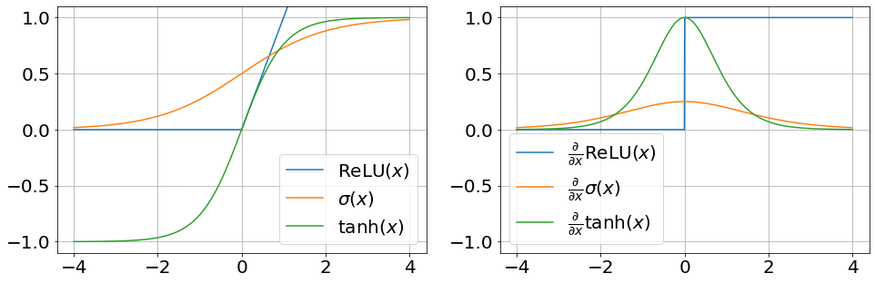

Why ReLU?

ReLU seems like a weird choice for a non-linearity, since it is actually linear for all positive inputs, and otherwise it’s just zero. But in practice it works very well. Some reasons for this are:

• Mitigates the vanishing gradients problem which traditionally prevented training deep networks with tanh or sigmoid activations. Since the gradient of ReLU is simply when , the gradient can be propagated back even in deep networks.
• Much faster to compute than sigmoid and tanh.
• Promotes sparse activations: some outputs get stuck as zero (causing “dead neurons”), which induces sparsity in the representations that these activations can produce.

Two-layer MLP from scratch

We’ll start our hands-on part by solving a simple regression problem with a 2-layer MLP (one hidden layer, one output layer). As in the previous post, we’ll start by implementing everything from scratch, including the gradient calculations, using numpy only, and graduate to a better pytroch-based implementation in the next section.

We’re trying to learn a continuous and perhaps non-deterministic target function .

The setup is as follows:

• Domain:
• Target:
• Model: , i.e. a 2-layer MLP, where:
  • sample (feature vector)
  • is the hidden dimension
  • We’ll set so output is a scalar
• Loss: MSE with L2 regularization,
• Optimization scheme: Vanilla SGD

Computing the gradients

Let’s write our model as

and manually derive the gradient of the point-wise loss using the chain rule.

Remember that to use SGD, we need the gradient of the loss w.r.t. our parameter tensors.

To continue into the nonlinearity, recall that we defined and that we apply the non-linearity elementwise on input tensors. Also, remember that the gradient of a vector w.r.t. another vector is the Jacobian, a matrix of mixed derivatives: .

In our case we have . Thus,

And so,

For the biases, we can easily see that:

The final gradients for weight update, including regularization will be

Implementation

The implementation will be straightforward, as we’ll directly incorporate the gradient derivations into our numpy code.

In this initial barebones version our model will actually be just a few tensors (two weight matrices and two bias vectors):

# N: batch size
# D_in: number of features
N, D_in =  64, 10
# H: hidden-layer
# D_out: output dimension
H, D_out =  100, 1
 
# Random input data
X = np.random.randn(N, D_in)
y = np.random.randn(N, D_out)
 
# Model weights and biases
wstd = 0.01
W1 = np.random.randn(H, D_in)*wstd
b1 = np.random.randn(H,)*wstd + 0.1
W2 = np.random.randn(D_out, H)*wstd
b2 = np.random.randn(D_out,)*wstd + 0.1
 
reg_lambda = 0.5
learning_rate = 1e-3

Now we can implement a training loop for our model. The training loop will implement our gradient calculation, and then update the model weights based on a negative gradient step.

losses = []
for epoch in range(250):
    # Forward pass, hidden layer: A = relu(X W1 + b1), Shape: (N, H)
    Z = X.dot(W1.T) + b1
    A = np.maximum(Z, 0)
    
    # Forward pass, output layer: Y_hat = A W2 + b2, Shape: (N, D_out)
    Y_hat = A.dot(W2.T) + b2
    
    # Loss calculation (MSE)
    loss = np.mean((Y_hat - y) ** 2); losses.append(loss) # (N, D_out)
    
    # Backward pass:  Output layer
    d_Y_hat = (1./N) * (Y_hat - y)     # (N, D_out)
    d_W2 = d_Y_hat.T.dot(A)            # (D_out, H)
    d_A = d_Y_hat.dot(W2)              # (N, H)
    d_b2 = np.sum(d_Y_hat, axis=0)     # (D_out,)
    
    # Backward pass: Hidden layer
    d_Z = d_A * np.array(Z > 0, dtype=np.float)  # (N, H)
    d_W1 = d_Z.T.dot(X)                          # (H, D_in)
    d_b1 = np.sum(d_Z, axis=0)                   # (H,)
    
    # Backward pass: Regularization term
    d_W2 += reg_lambda * W2
    d_W1 += reg_lambda * W1
    
    # Gradient descent step
    W2 -= d_W2 * learning_rate; b2 -= d_b2 * learning_rate
    W1 -= d_W1 * learning_rate; b1 -= d_b1 * learning_rate
    print('.', end='')

Running the above and plotting, we get:

_, ax = plt.subplots(figsize=(10,5))
ax.plot(losses)
ax.set_ylabel('MSE loss'); ax.set_xlabel('Epoch');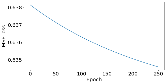

Note that this implementation is not ideal (read: very bad), as it’s:

• Non modular (hard to switch components)
• Hard to extend (e.g. to add layers)
• Error prone (hard-coded manual calculations)

But, it works! now, we’ll see how to address these issues using some of pytorch’s functionality.

N-Layer MLP using PyTorch

This time we’ll create a more modular implementation where each of thes the core components (dataset, model, loss function, optimizer) is separate and can be changed independently of the others. We’ll also leverage pytorch’s autograd feature to compute the gradients without us having to re-derive them for an N-layer model.

Dataset

As in the previous post we’ll tackle an image classification task, the MNIST database of handwritten digits.

import torch
import torch.utils.data
import torchvision
import torchvision.transforms
 
root_dir = os.path.expanduser('~/.pytorch-datasets/')
batch_size = 512
train_size = batch_size * 10
test_size = batch_size * 2

We’ll create the standard built-in pytorch datasets and loaders, and load one sample from the dataset to see its shape.

# Datasets and loaders
tf_ds = torchvision.transforms.ToTensor()
ds_train = torchvision.datasets.MNIST(root=root_dir, download=True, train=True, transform=tf_ds)
dl_train = torch.utils.data.DataLoader(ds_train, batch_size,
                                       sampler=torch.utils.data.SubsetRandomSampler(range(0,train_size)))
ds_test =  torchvision.datasets.MNIST(root=root_dir, download=True, train=False, transform=tf_ds)
dl_test = torch.utils.data.DataLoader(ds_test, batch_size,
                                       sampler=torch.utils.data.SubsetRandomSampler(range(0,test_size)))
 
x0, y0 = ds_train[0]
n_features = torch.numel(x0)
n_classes = 10
 
print(f'x0: {x0.shape}, y0: {y0}')

x0: torch.Size([1, 28, 28]), y0: 5

Let’s look at the first few images in this dataset and also show the labels.

import sys
sys.path.append('..')
import t02.plot_utils as plot_utils
 
# Show first few samples
plot_utils.dataset_first_n(ds_train, 10, cmap='gray', show_classes=True);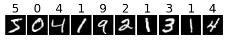

Model Implementation

In this section, we’ll look at various parts of the torch.nn API. The torch.nn module contains building blocks such as neural network layers, loss functions, activations and more. Specifically,

• We’ll use nn.Linear which implements a single MLP layer.
• We’ll implement our model as a subclass of nn.Module, which means:
  • Any tensors we set as properties will be registered as model parameters.
  • We can nest nn.Modules and get all model parameters from the top-level nn.Module.
  • Can be used as a function if we implement the forward() method.

The nn.Module class

The nn.Module class will be our base class for implementing pytorch-based models. To understand nn.Module, lets look at a very basic one: the fully-connected layer.

import torch.nn as nn
 
fc = nn.Linear(in_features=3, out_features=5, bias=True)
 
# Input tensor with 10 samples of 3 features
t = torch.randn(10, 3)
 
# Forward pass, notice that grad_fn exists
fc(t)

tensor([[-7.1251e-01,  8.1881e-01,  7.9059e-01, -2.7722e-01, -1.2208e-01],
        [ 1.5439e-01, -1.8635e-04, -9.3113e-02,  2.2336e-01,  1.2809e-01],
        [-7.7973e-01,  2.9552e-02,  1.0179e+00, -3.1256e-01,  3.1589e-01],
        [ 9.4211e-02,  1.2330e+00,  1.1839e-01, -4.2630e-01, -8.4664e-01],
        [ 1.0505e+00, -1.0999e+00, -6.8395e-01,  2.8644e-01,  2.7877e-01],
        [-2.4097e-01, -3.0381e-01,  4.5856e-01, -3.9520e-02,  3.5719e-01],
        [ 1.7276e-01, -5.4743e-02,  8.5343e-02, -8.0329e-02, -1.4909e-02],
        [ 4.7882e-01,  1.0415e-01, -4.0715e-01,  2.5505e-01, -8.1025e-02],
        [-9.6874e-01,  1.2249e+00,  1.1322e+00, -6.0926e-01, -3.8214e-01],
        [-1.2650e-01,  6.5705e-01,  3.9818e-01, -3.9975e-01, -4.0890e-01]],
       grad_fn=<AddmmBackward>)

nn.Modules have registered parameters, which are tensors which require_grad.

# Note parameter shapes
for i, param in enumerate(fc.parameters()):
    print(f"Parameter #{i} of shape {param.shape}:\n{param.data}\n")

Parameter #0 of shape torch.Size([5, 3]):
tensor([[ 0.5771, -0.0683,  0.1145],
        [-0.3558,  0.5217,  0.2677],
        [-0.5193,  0.2295, -0.2657],
        [ 0.1603, -0.4462,  0.1953],
        [-0.0272, -0.4815, -0.0986]])

Parameter #1 of shape torch.Size([5]):
tensor([-0.1998,  0.2915,  0.3349, -0.0784, -0.0032])

We can create custom nn.Modules with arbitrary logic. To demonstrate this, let’s implement a fully-connected layer ourselves (although pytorch of course has an implementation).

class MyFullyConnectedLayer(nn.Module):
    def __init__(self, in_features, out_features):
        super().__init__() # don't forget this!
        # nn.Parameter just marks W,b for inclusion in list of parameters
        self.W = nn.Parameter(torch.randn(out_features, in_features, requires_grad=True))
        self.b = nn.Parameter(torch.randn(out_features, requires_grad=True))
                
    def forward(self, x):
        # x assumed to be (N, in_features)
        z = torch.matmul(x, self.W.transpose(0, 1)) + self.b
        # For no good reason, our custom layer multiplies outputs by 3
        return 3*z

myfc = MyFullyConnectedLayer(in_features=3, out_features=5)
myfc(t)

tensor([[ -4.7093,   4.2600,   1.8041,   0.0312,  -1.6802],
        [ -3.1112,  -2.5073,  -3.9814,   5.2684,   5.1788],
        [ -2.2845,  -7.8631,   7.4091,   3.0125,   2.5034],
        [ -5.3586,   7.2746, -10.1273,   1.1065,  -1.4891],
        [  0.3269, -19.3289,  -8.0095,  12.3404,  13.9024],
        [ -1.7318,  -9.9620,   2.7862,   5.6232,   5.8142],
        [ -2.2552,  -7.3950,  -3.5877,   5.9778,   5.6912],
        [ -3.3929,  -0.9995,  -8.4880,   5.8171,   5.5529],
        [ -5.2573,   6.2478,   2.6922,  -1.9056,  -4.5206],
        [ -3.7618,  -0.6266,  -4.0507,   2.6731,   1.0251]],
       grad_fn=<MulBackward0>)

The class instances of type nn.Parameter are automatically registered as model parameters and exposed via a dedicated function:

list(myfc.parameters())

[Parameter containing:
 tensor([[ 0.2957, -0.1923, -0.4026],
         [-1.3305,  0.6385,  2.1411],
         [-1.6123, -0.6444, -1.0526],
         [ 0.9936, -0.5495, -0.3296],
         [ 1.2023, -0.9536, -0.4132]], requires_grad=True),
 Parameter containing:
 tensor([-1.1385, -0.5594, -0.4224,  1.1462,  0.8879], requires_grad=True)]

Quick visualization of our custom module’s computation graph. Notice that it represents all the steps in our layers computation, including the superfluous multiplication we added at the end.

import torchviz
torchviz.make_dot(myfc(t), params=dict(W=myfc.W, b=myfc.b))

Custom MLP

Now that we know about nn.Modules, we can create a fairly-general MLP for multiclass classification.

class MLP(torch.nn.Module):
    NLS = {'relu': torch.nn.ReLU, 'tanh': nn.Tanh, 'sigmoid': nn.Sigmoid, 'softmax': nn.Softmax, 'logsoftmax': nn.LogSoftmax}
 
    def __init__(self, D_in: int, hidden_dims: Sequence[int], D_out: int, nonlin='relu'):
        super().__init__()
        
        all_dims = [D_in, *hidden_dims, D_out]
        non_linearity = MLP.NLS[nonlin]
        layers = []
        
        for in_dim, out_dim in zip(all_dims[:-1], all_dims[1:]):
            layers += [
                nn.Linear(in_dim, out_dim, bias=True),
                non_linearity()
            ]
        
        # Sequential is a container for layers
        self.fc_layers = nn.Sequential(*layers[:-1])
        
        # Output non-linearity
        self.log_softmax = nn.LogSoftmax(dim=1)
 
    def forward(self, x):
        x = torch.reshape(x, (x.shape[0], -1))
        z = self.fc_layers(x)
        y_pred = self.log_softmax(z)
        # Output is always log-probability
        return y_pred

Create an instance of the model: 5-layer MLP, and show it’s architecture:

mlp5 = MLP(D_in=n_features, hidden_dims=[32, 64, 128, 64], D_out=n_classes, nonlin='tanh')
print(mlp5)

MLP(
  (fc_layers): Sequential(
    (0): Linear(in_features=784, out_features=32, bias=True)
    (1): Tanh()
    (2): Linear(in_features=32, out_features=64, bias=True)
    (3): Tanh()
    (4): Linear(in_features=64, out_features=128, bias=True)
    (5): Tanh()
    (6): Linear(in_features=128, out_features=64, bias=True)
    (7): Tanh()
    (8): Linear(in_features=64, out_features=10, bias=True)
  )
  (log_softmax): LogSoftmax(dim=1)
)

Parameter tensors are automatically discovered, even in nested nn.Modules:

print(f'number of parameter tensors: {len(list(mlp5.parameters()))}')

number of parameter tensors: 10

print(f'number of parameters: {np.sum([torch.numel(p) for p in mlp5.parameters()])}')

number of parameters: 44458

Let’s check that a forward pass works:

y_hat0 = mlp5(x0)
 
print(f'{x0.shape=}\n')
print(f'{y_hat0.shape=}\n')
print(f'{y_hat0=}')

x0.shape=torch.Size([1, 28, 28])

y_hat0.shape=torch.Size([1, 10])

y_hat0=tensor([[-2.2561, -2.4066, -2.4193, -2.2582, -2.2500, -2.2905, -2.2327, -2.2299,
         -2.4094, -2.2993]], grad_fn=<LogSoftmaxBackward>)

And finally, repeat the computation graph visualization, for our full MLP:

torchviz.make_dot(mlp5(x0), params=dict(mlp5.named_parameters()))

Loss and Optimizer

For the loss function, we can use PyTorch’s built in negative log-likelihood loss since our model outputs probabilities.

import torch.optim
 
# Loss: assumes *log*-probabilities (given by our LogSoftmax layer)
loss_fn = nn.NLLLoss()
 
# Fake labels (no need to 1-hot encode)
yt = torch.randint(low=0, high=n_classes, size=(y_hat0.shape[0],))
 
# Try out the loss
loss_fn(y_hat0, yt) 

tensor(2.2582, grad_fn=<NllLossBackward>)

Note that nn.NLLLoss(y_hat, y) assumes that , where contains the raw scores for input , and therefore it simply computes:

where is the ground-truth class label of for sample .

As for the optimization scheme, we’ll use a built in SGD optimizer from the torch.optim module. We will see that the semantics of using it are similar to the simple optimizer we previously implemented from scratch. Specifically, the pytorch optimizers are instantiated using a model’s parameters, which are usually exposed automatically from the parameters() method of any nn.Module.

The best thing about using pytorch is that we won’t need to calculate the loss gradient this time, as we’ll use autograd for automatic differentiation.

torch.manual_seed(42)
 
# Model for training
model = MLP(D_in=n_features, hidden_dims=[32, 32, 32], D_out=n_classes, nonlin='relu')
 
# Optimizer: instantiated using our model's parameters
optimizer = torch.optim.SGD(params=model.parameters(), lr=5e-2, weight_decay=0.01, momentum=0.9)

Training loop

This time we’ll train over lazy-loaded batches from our data loader instead of loading the entire dataset into memory up-front (which clearly isn’t feasible beyond toy datasets).

Notice that except for our model’s __init__() and __forward()__, we’re using PyTorch facilities for the entire training implementation.

num_epochs = 10
for epoch_idx in range(num_epochs):
    total_loss = 0
    
    for batch_idx, (X, y) in enumerate(dl_train):
        # Forward pass
        y_pred = model(X)
 
        # Compute loss
        loss = loss_fn(y_pred, y)
        total_loss += loss.item()
 
        # Backward pass
        optimizer.zero_grad() # Zero gradients of all parameters
        loss.backward()       # Run backprop algorithms to calculate gradients
        
        # Optimization step
        optimizer.step()      # Use gradients to update model parameters
        
    print(f'Epoch #{epoch_idx+1}: Avg. loss={total_loss/len(dl_train)}')

Epoch #1: Avg. loss=2.305134320259094
Epoch #2: Avg. loss=2.2864507913589476
Epoch #3: Avg. loss=2.256749725341797
Epoch #4: Avg. loss=2.176988220214844
Epoch #5: Avg. loss=1.9311089158058166
Epoch #6: Avg. loss=1.4161055207252502
Epoch #7: Avg. loss=0.9191412627696991
Epoch #8: Avg. loss=0.676337045431137
Epoch #9: Avg. loss=0.5613921701908111
Epoch #10: Avg. loss=0.5014605939388275

The most crucial part in this training loop are the three magical lines at the end. Lets go through them:

1. optimizer.zero_grad(): This sets the gradients of all the parameter tensors to zero.
   • Each pytorch tensor has both a .data and a .grad attribute. We need to clear the gradients that are still there from the previous batch.
   • This is done via the optimizer, which has access to all the relevant parameter tensors from the model.
2. loss.backward(): This is the backward pass, where the magic of autograd happens.
   • Recall that the loss tensor here is the output of some computation graph, specifically the one we visualized above.
   • Using the back-propagation algorithm, autograd goes back through the graph, finds each parameter tensor involved in the calculation, and calculates the gradient of the loss with respect to that parameter.
   • This gradient then populates the .grad attribute of each parameter tensor.
3. optimizer.step(): Here we update the model parameters based on their gradients.
   • Thanks to the backward pass, now the .grad attribute of each parameter tensor is populated.
   • Each optimizer implements a different algorithm, but generally all of them need to change the model parameters slightly in the direction of the negative gradient.
   • For each parameter tensor, the optimizer with update its .data using the value in .grad. See the simple SGDOptimizer we implemented previously for an idea of what happens here.

Note that the order of the above operations is crucial: If we don’t zero the gradients before the backward pass, the optimizer’s step would then update the parameters using incorrect gradients.

Conclusion

Using the basic PyTorch building blocks we have arrived at a much more robust implementation. It’s now much easier to:

• Change architecture: add layers and activation functions
• Change loss: we can can instantiate another loss function and pass it into the training loop
• Change optimization method: any pytorch optimizer could’ve been used here.

And most importantly, there’s no need for manual gradient derivations. We could implements arbitrary layers and logic, and all this gets encoded as a computation graph which autograd can then use for gradient calculations.