Introduction
In this post we’ll explore an alternative to RNNs for working with sequence-based or time-series data: Temporal convolution networks (TCNs), which were proposed in a recent paper (Bai et al., 2018). TCNs are actually just 1D CNNs, with some key hyperparameter choices. We’ll see how CNNs can be used for modeling sequences, and how this approach mitigates both drawbacks of RNNs.
Concretely, this post will cover:
- Adapting CNNs to the special considerations required to work with sequences
- Implementing a TCN from scratch
- Using a TCN-based model as an alternative to an RNN for a simple sentiment classification task
References
This post is based on materials created by me for the CS236781 Deep Learning course at the Technion between Winter 2019 and Spring 2022. To re-use, please provide attribution and link to this page.
Some images used here were taken and/or adapted from the following sources:
- Bai et al. 2018, http://arxiv.org/abs/1803.01271
Background: the limitations of RNNs
In a previous post, I covered how RNNs can be used as a deep learning model for input sequences. Despite their conceptual simplicity, we saw that RNNs suffer for some serious drawbacks:
- They require their input sequence to be provided one element at a time. This results in poor performance in both training and inference, and limits the ability to exploit parallelization.
- They struggle to train with with long sequences due to vanishing/exploding gradients. These can happen with any model, but are especially likely to arise in RNNs due to backpropagation through time.
CNNs, on the other hand, are great on these fronts! They are easy to train even with very deep architectures (especially when residual connections are used), and they have very efficient implementations, because convolutions can be implemented as matrix multiplications leveraging low-level hardware parallelization.
Can we somehow use CNNs to process sequences of arbitrary length?
Processing sequences with CNNs
It turns out that we can indeed leverage CNNs for sequence modeling. To make it work, we’ll need to handle three things in particular:
- Input and output must both be sequences of the same length, which should be arbitrary.
- Output at time
should depend solely on inputs up to time . - Long-range dependencies across time should be supported.
Before reading on, I encourage you to make sure you understand what fully-convolutional architectures are, and how hyperparameters affect the output shape in a CNN model. Both topics are covered in the linked previous post.
Let’s now see how to handle each of these challenges.
1. Arbitrary input/output length
To work with sequences, the input and outputs must both be sequences of the same length, which should be arbitrary.
We have already discussed how CNNs are actually flexible in the spatial dimension (height and width of the input image), and only need to know the number of input channels up front.
The trick to working with sequences therefore simply boils down to these things:
- Treating the sequence
as the CNN’s “spatial” dimension, and the embedding dimension as “channels”. - Using a 1D fully-convolutional architecture.
- Selecting a hyperparameter combination (kernel size, padding, strides, dilation) that maintains the spatial extent of the input.
To see this, imagine applying a CNN layer to an image that’s just a single row of pixels (
Furthermore, by choosing an appropriate padding and strides for a given kernel size, we maintain the spatial extent of the input. So for example, if we use a
Note that in practice, we don’t need to treat the input as a single-row image and use a Conv1d directly handles this case. The image analogy was just for re-using the intuition you might already have about 2D convolutions.
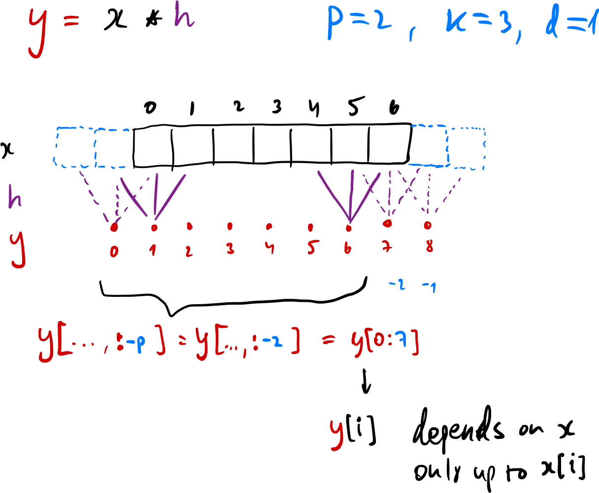
2. Maintaining causality
In a vanilla RNN, the output at time
The solution here is to use causal convolutions, where an output at time
In practice this can be achieved simply by applying a regular convolution with a particular choice of padding, and then just sliding the output to only the causal part:
- The padding should be chosen as
where is the kernel size and is the dilation. - After applying each individual convolution
, slice out the causal part via .
This approach maintains the input’s spatial extent (which is now the sequence length), while also ensuring that each output element was only computed from elements which are no later in time. To see why this works, see the figure below (sorry for hand-drawing…).
3. Modeling long-range dependencies across time
RNNs model long-range dependencies across time via passing of the hidden-state vector. This means that a late output (say
With CNNs, each output “pixel” is a function of the input pixels that appeared in its receptive field.
We can increase the receptive field using deeper networks (more CNNs layers, often requiring residual connections), larger kernel sizes, and dilated convolutions.
Using dilation is an especially effective way to control the receptive field. For example, a dilation factor that doubles between layers causes the receptive field to grow exponentially. Deep CNNs with dilation can therefore quickly create large receptive fields that allow modeling long-range temporal behavior often required for signal processing applications.
For a TCN with
Putting it all together
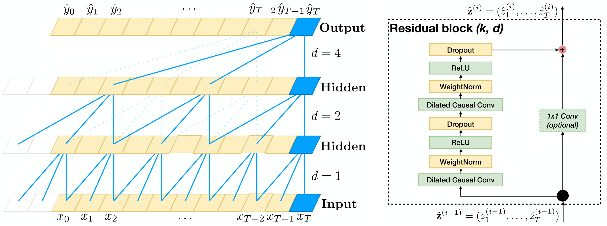
Combining the three techniques discussed above, gives us the TCN architecture proposed by Bai et al. (2018). The figure below shows the architecture. The key points clearly visible in the figure are:
- 1D convolutions with padding and output slicing to ensure causality and a consistent output sequence size.
- Dilation doubles each layer: for layer
, . - Residual skip connections to support deep CNNs that can be trained easily.
TCN Implementation
Let’s implement a general TCN residual block from scratch, by incorporating all the implementation details discussed above. The implementation should be straightforward to follow once you understand the previous points.
class TCNBlock(nn.Module):
    def __init__(self, in_channels, out_channels, kernel_size, dilation, dropout=0.2):
        super().__init__()

        # Control padding to maintain causal output size for a fixed kernel size
        padding = (kernel_size - 1) * dilation

        self.conv1 = nn.Sequential(
            nn.Conv1d(in_channels, out_channels, kernel_size, stride=1, padding=padding, dilation=dilation),
            nn.ReLU(),
            nn.Dropout(dropout)
        )
        self.conv2 = nn.Sequential(
            nn.Conv1d(out_channels, out_channels, kernel_size, stride=1, padding=padding, dilation=dilation),
            nn.ReLU(),
            nn.Dropout(dropout)
        )
        if in_channels != out_channels:
            self.channels_adapter = nn.Conv1d(in_channels, out_channels, kernel_size=1)
        else:
            self.channels_adapter = None

        self.padding = padding

    def forward(self, x):
        # Main branch
        out = self.conv1(x)
        out = out[..., :-self.padding] # slice to maintain causality
        out = self.conv2(out)
        out = out[..., :-self.padding]

        # Skip-connection (residual branch)
        skip = x if not self.channels_adapter else self.channels_adapter(x)
        out = out + skip
        return out
Here’s what a small TCN block looks like:
TCNBlock(in_channels=2, out_channels=4, kernel_size=3, dilation=1)TCNBlock(
(conv1): Sequential(
(0): Conv1d(2, 4, kernel_size=(3,), stride=(1,), padding=(2,))
(1): ReLU()
(2): Dropout(p=0.2, inplace=False)
)
(conv2): Sequential(
(0): Conv1d(4, 4, kernel_size=(3,), stride=(1,), padding=(2,))
(1): ReLU()
(2): Dropout(p=0.2, inplace=False)
)
(channels_adapter): Conv1d(2, 4, kernel_size=(1,), stride=(1,))
)
Notice the channel_adapter blocks that we added. Why are they required? They allow the residual skip-connections to skip over CNNs layers with a different number of output channels. These adapters are simply 1D convolutions placed on the skip connections that project the input number of channels up/down to match the number of channel that the skip connection needs to be added to.
TCN-based sentiment classifier
Using our custom TCN block, we can now implement a full TCN-based model for the same sentiment analysis task that we previously solved with an RNN. For the data loading and processing (tokenization, embedding, vocabulary construction), and the training loop implementation, please refer to the relevant section of my previous post.
The model implementation is quite straightforward. We’ll instantiate a TCNBlock for each layer, making sure to increase the dilation by a factor of 2 each time. In the forward pass, we first embed our token sequence to a sequence of dense vectors (as before). We then just need to reshape the result into the shape that a 1D CNN expects, so that the sequence becomes the “spatial” dimension, and the embedding dimension becomes the “channels”.
class SentimentTCN(nn.Module):
    def __init__(self, vocab_dim: int, embedding_dim: int, layer_channels: list, out_dim: int, kernel_size=3, dropout=0.2):
        super().__init__()
        assert len(layer_channels) > 0

        self.embedding = nn.Embedding(vocab_dim, embedding_dim)

        tcn_channels = [embedding_dim] + layer_channels + [out_dim]
        layers = []
        for i, (c_in, c_out) in enumerate(zip(tcn_channels[:-1], tcn_channels[1:])):

            # Exponentially-increasing dilation
            dilation = 2 ** i

            layers.append(
                TCNBlock(c_in, c_out, kernel_size, dilation=dilation, dropout=dropout)
            )

        self.blocks = nn.Sequential(*layers)
        self.log_softmax = nn.LogSoftmax(dim=1)

    def forward(self, x, **kw): # x is (S, B)
        # First we need to embed our sequence.
        # Note how we treat the E as channels for the convolutions.
        x_emb = self.embedding(x) # (S, B, E)
        x_emb = torch.transpose(x_emb, 0, 1) # (B, S, E)
        x_emb = torch.transpose(x_emb, 1, 2) # (B, E, S)

        # Process the entire sequence (at once!)
        y_seq = self.blocks(x_emb) # (B, D_out, S)

        # Output predictions
        yt = y_seq[..., -1] # (B, D_out)
        yt_log_proba = self.log_softmax(yt)
        return yt_log_proba
Let’s instantiate it and look at the architecture.
tcn = SentimentTCN(INPUT_DIM, EMBEDDING_DIM, [32, 32], OUTPUT_DIM, kernel_size=3)
tcn
SentimentTCN(
(embedding): Embedding(15482, 100)
(blocks): Sequential(
(0): TCNBlock(
(conv1): Sequential(
(0): Conv1d(100, 32, kernel_size=(3,), stride=(1,), padding=(2,))
(1): ReLU()
(2): Dropout(p=0.2, inplace=False)
)
(conv2): Sequential(
(0): Conv1d(32, 32, kernel_size=(3,), stride=(1,), padding=(2,))
(1): ReLU()
(2): Dropout(p=0.2, inplace=False)
)
(channels_adapter): Conv1d(100, 32, kernel_size=(1,), stride=(1,))
)
(1): TCNBlock(
(conv1): Sequential(
(0): Conv1d(32, 32, kernel_size=(3,), stride=(1,), padding=(4,), dilation=(2,))
(1): ReLU()
(2): Dropout(p=0.2, inplace=False)
)
(conv2): Sequential(
(0): Conv1d(32, 32, kernel_size=(3,), stride=(1,), padding=(4,), dilation=(2,))
(1): ReLU()
(2): Dropout(p=0.2, inplace=False)
)
)
(2): TCNBlock(
(conv1): Sequential(
(0): Conv1d(32, 3, kernel_size=(3,), stride=(1,), padding=(8,), dilation=(4,))
(1): ReLU()
(2): Dropout(p=0.2, inplace=False)
)
(conv2): Sequential(
(0): Conv1d(3, 3, kernel_size=(3,), stride=(1,), padding=(8,), dilation=(4,))
(1): ReLU()
(2): Dropout(p=0.2, inplace=False)
)
(channels_adapter): Conv1d(32, 3, kernel_size=(1,), stride=(1,))
)
)
(log_softmax): LogSoftmax(dim=1)
)
Let’s see how many parameters we have.
print(f'The TCN model has {count_parameters(tcn):,} trainable weights.')The TCN model has 1,570,796 trainable weights.
We’ll try a forward pass with this new model, making sure the output shape looks correct:
tcn(X)tensor([[-1.0986, -1.0986, -1.0986],
[-1.1709, -0.9898, -1.1450],
[-1.0986, -1.0986, -1.0986],
[-1.1102, -1.1102, -1.0759]], grad_fn=<LogSoftmaxBackward>)
Finally, we can train the new model using the same setting and training loop as we used before.
tcn_model = SentimentTCN(INPUT_DIM, EMBEDDING_DIM, [32, 32], OUTPUT_DIM, kernel_size=3)
optimizer = optim.Adam(tcn_model.parameters(), lr=1e-4)
loss_fn = nn.NLLLoss()

train(tcn_model, optimizer, loss_fn, dl_train, max_epochs=4)
Epoch #0, loss=1.075, accuracy=0.390, elapsed=3.7 sec
Epoch #1, loss=1.061, accuracy=0.396, elapsed=3.5 sec
Epoch #2, loss=1.053, accuracy=0.398, elapsed=3.5 sec
Epoch #3, loss=1.034, accuracy=0.427, elapsed=3.8 sec
Comparison to the RNN-based approach
To contrast this new approach with the previous RNN-based approach, notice how the model still works with sequences of different length every batch, just like an RNN. However, here the sequences were processed in parallel w.r.t. time, unlike in the RNN case where we needed an explicit loop over tokens in the forward pass, which is much slower.
In the TCN, the receptive field was determined by architecture choices, which we control. This is both a strength (because we control it) and a limitation: if a sequence is longer than the receptive field, distant inputs simply can’t influence the output. With the RNN, the receptive field was determined by the sequence length, which we don’t control. However, the hidden state theoretically allows arbitrarily long dependencies, although vanishing gradients make it hard to exploit in practice.
Finally, with the TCN approach there was no need for backpropagation through time, since this is a standard feedforward architecture, where we just have regular backpropagation through multiple CNN layers.
Conclusions
TCNs provide a way to model sequences without the need for recurrence. The core ideas were actually quite simple: 1D convolutions, making them causal with padding and slicing, and exploiting exponentially growing dilation to create a large receptive field. The resulting model processes sequences in parallel, has a well-defined and controllable receptive field, and avoids the vanishing/exploding gradient issues of backpropagation through time.
On our toy sentiment task, the TCN was comparable to the vanilla RNN, since both models were deliberately kept simple. In practice, TCNs have been shown to match or exceed the performance of LSTMs and GRUs across a range of benchmarks (Bai et al., 2018).
Both RNNs and TCNs are increasingly being replaced by transformers, particularly in the domain of NLP. However, TCNs are arguably simpler, and more performant than transformers. This means that TCNs could remain practical and relevant in signal processing and time-series applications where causality and computational efficiency are important.