Introduction
In this post, we will tackle an application that’s simple to grasp, yet not trivial to solve. Given a sentence written in some natural language, how can we classify the sentiment it conveys into “positive”, “negative” or “neutral”?
To solve this with deep learning, we’ll need to learn how to work with text, and we’ll need models that support inputs of arbitrary length (rather than just fixed-length feature vectors or images). We’ll do it with recurrent neural networks (RNNs). RNNs have been going out of fashion in recent years, slowly being replaced by TCNs or attention-based models (transformers). However, RNNs are still quite interesting, and I found that learning about them helped me solidify my understanding of deep learning in general. I hope this post will do the same for you.
This is a hands-on post which will focus mainly on how to implement a full solution, while keeping it as simple and minimal as I can. Concretely, we’ll focus on:
- What recurrent neural networks (RNNs) are and how they work
- Special considerations and limitations of back-propagation with RNNs
- Implementing a basic RNNs from scratch with pytorch
- Using RNNs to classify the sentiment of movie reviews
References
This post is based on materials created by me for the CS236781 Deep Learning course at the Technion between Winter 2019 and Spring 2022. To re-use, please provide attribution and link to this page.
Some images used here were taken and/or adapted from the following sources:
- Fundamentals of Deep Learning, Nikhil Buduma, Oreilly 2017
- Sebastian Ruder, “On word embeddings - Part 1”, 2016, https://ruder.io
- Andrej Karpathy, http://karpathy.github.io
- MIT 6.S191
- Stanford cs231n
- Alex Bronstein’s deep learning course lecture slides
Background
To understand this post, make sure you’re familiar with the basic building blocks of deep learning models, and how to train them. See my previous posts about MLPs and CNNs for a detailed overview. For convenience, here are the most-relevant basics.
Quick recap: linear and convolutional layers
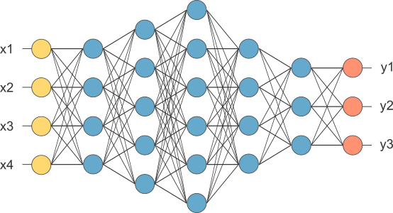
Fully connected layers:
- Each layer
operates on the output of the previous layer ( ) and calculates, - FCs have completely fixed input and output dimensions, which must be known a-priori.
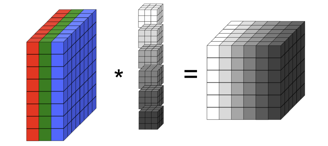
Convolutional layers:
- Each layer operates on an input tensor
containing feature maps. - The
-th feature map of the output tensor is: Where denotes convolution, and is the number of output feature maps.
- The weight dimensions are not dependent on the input dimensions.
- Weights are shared across the spatial dimensions of the input.
- Output spatial dimension can change based on input spatial dimension, but the input number of channels must be known a-priori.
The problem with sequences
What happens when our input is naturally a sequence or time series? For example, consider an autoregressive model, i.e.
In such a system, the output
In more complicated cases, the number of past inputs or outputs that need to be considered might also change between different examples. For example, a text classifier must support an input sequence containing an arbitrary number of words. Therefore, in addition to memory, we also need a way to support variable length input/output sequences.
These cases arise in many domains, such as signal processing, text translation or classification, scene classification in video, etc, and clearly highlight two key limitations of MLP and CNN models. First, both these models have no state (or memory) that persists between inputs. In other words, the current output is not affected by previous inputs (or outputs). Second, their input size needs to be known in advance. For MLPs, the exact number of input features must be baked into the architecture. For CNNs, the number of input channels be fixed. CNNs are more flexible though because the spatial size of the input (height, width) can be variable (but only in fully-convolutional architectures, and usually, it can only be larger than some base size).
We have noted that CNNs allow sharing weights across space: the same convolutional filter is applied at various positions in an image, and thus it can detect a shape regardless of its spatial position. Likewise, we’ll see how RNNs allow sharing weights across time, applying the same learned function to different parts of the input sequence. We’ll see that this is the key to solving the two limitations stated above.
Recurrent layers
An RNN layer is similar to a regular FC layer, but it has two inputs:
- Current sample,
. - Previous state,
.
Given these inputs, it then produces two outputs which depend on both:
- Current layer output,
. - Current state,
.
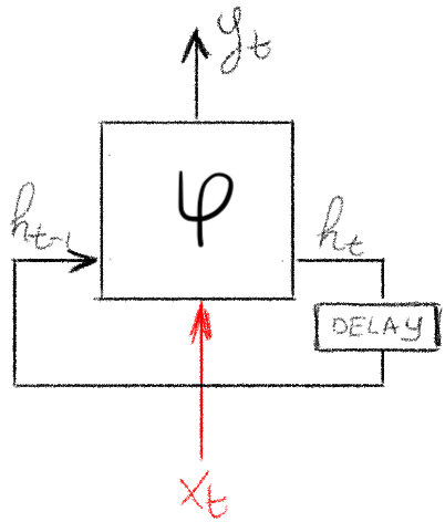
Crucially, the layer itself is not time-dependent: the same function is applied at successive time steps, just on different inputs and state. Of course, we are in the context of deep learning, so this function will have parameters that can be tuned via optimization.
A basic RNN can be defined using a few linear layers, as follows:
Where,
is the input at time . is the previous hidden state, i.e. from time . is the output at time . , , , and are the model weights and biases. Each weight matrix (with optional bias vector) is just a regular linear layer. and are some non-linear functions. The is optional and is sometimes not used.
Modeling time-dependence
We can now imagine unrolling a single RNN layer through time. This simply means that we take a sequence of input vectors 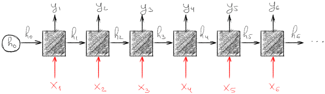
We can see that late outputs can now be influenced by early inputs, through the hidden state. At each time step, we’re just applying the same function (with the same tunable weight vectors), but on different inputs. Passing the hidden state vector maintains a temporal link between the inputs.
RNN models are very flexible in terms of input and output meaning. For example, after feeding in
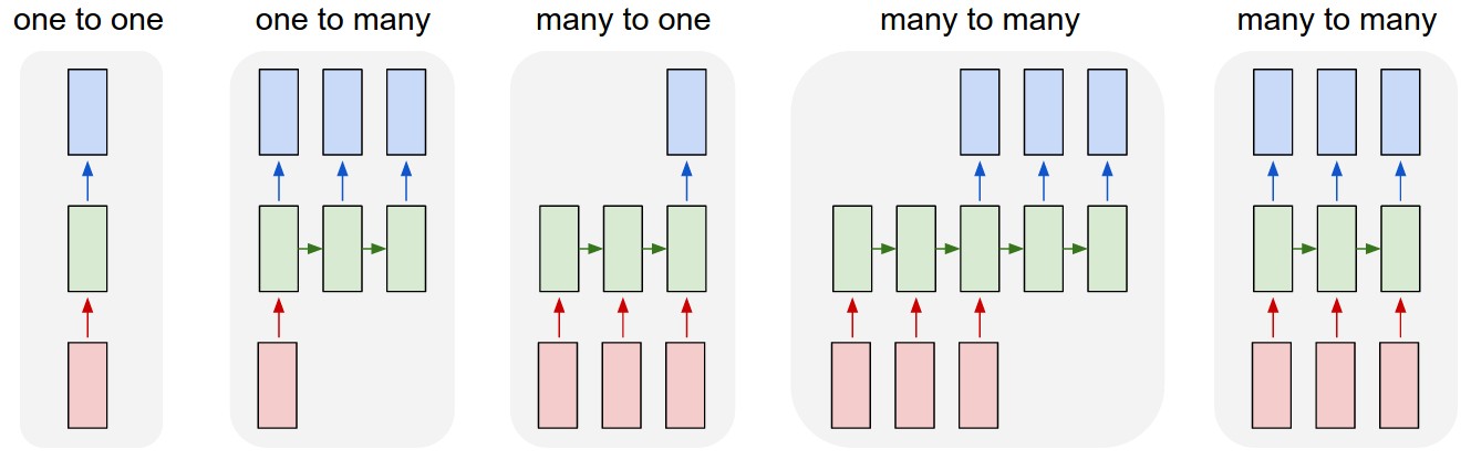
Backpropagation through time
How does training work for RNNs? As usual, we need to back-propagate to compute the gradient of some loss with respect to each parameter, and use these gradient to update the model (see my post on optimization basics for a recap).
With a regular MLP, we might have to propagate the gradient back through several layers. The gradient for each layer depends on the layers that came after it in the forward pass, due to the application of the chain rule. Each MLP layer has a different set of parameters, and we obtain the gradient of the loss w.r.t. each.
In the case of an RNN, we still have just one set of parameters per layer, but we applied them more than once. In fact, we apply these parameters
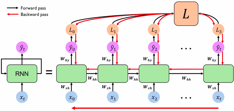
When we compute the gradient of a sum, we sum the gradients. In this case, it means we need to sum the gradients from each time
This is known as backpropagation through time, or BPTT. If we denote all the parameters of the layer collectively as
Notice how we use the chain rule to go back through the chain of
What does each Jacobian
where
Finally, the total gradient is then the simply sum
How far back should we go?
What’s the limiting factor for BPTT? Can we really expect to be able to back-propagate through arbitrarily long sequences?
The issue starts with the product
If the magnitudes of the eigenvalues of these Jacobians are consistently less than 1, the product shrinks exponentially with each multiplication. This would cause gradients from distant past times to vanish, and the model would fail to learn long-range temporal dependencies. If they’re consistently greater than 1, the product grows exponentially. Gradients would explode, making training unstable (although in practice we could clip the gradient to some maximal norm).
The choice of activation also contributes to the problem. For example, with
Unlike in a regular feedforward network, where each layer has its own weights, in an RNN the same
These issues motivated the development of more advanced RNN architectures (LSTMs and GRUs), which add paths which gradients can flow through without this repeated product.
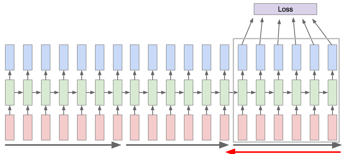
One pragmatic solution is to limit the number of time steps involved in the backpropagation. We can simply decide not to go all the way back to
Multi-layered (deep) RNN
RNNs layers can be stacked to build a deep RNN model.
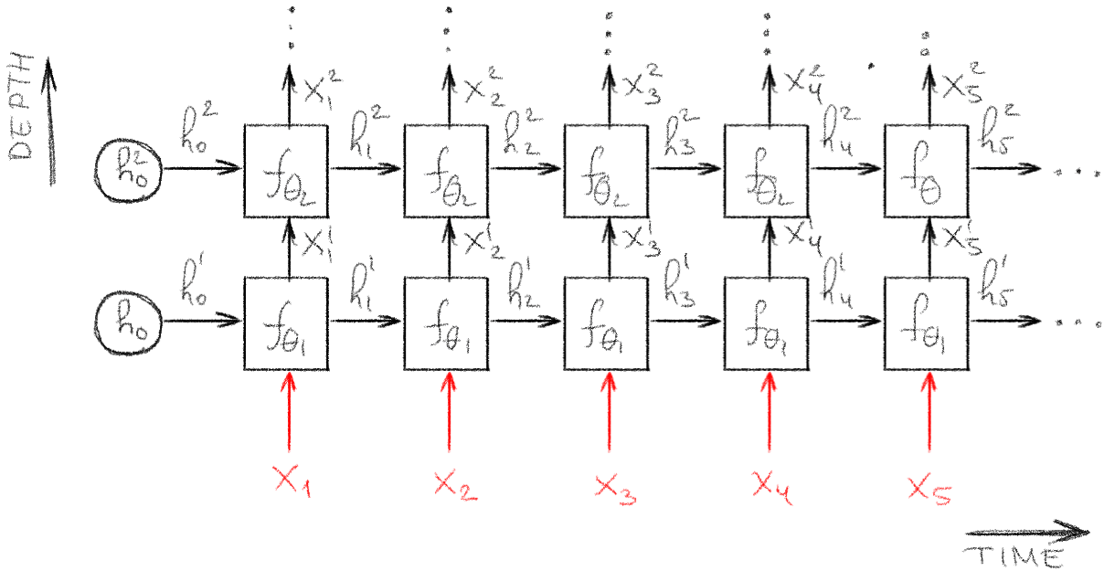
As with MLPs, adding depth allows us to learn intricate hierarchical features, which are produced as the output at each time. Moreover, this also makes the hidden state vectors highly non-linear function, which could potentially convey more detailed information between the consecutive time steps.
However, from an optimization perspective, this deeper architecture could exacerbate training stability issues, since we need to back-propagate both through time and also though multiple layers at each time.
RNN Implementation
We can now create a simple RNN layer with PyTorch. To keep it clear and simple, we’ll implement it from scratch, exactly based on the equations above.
To represent the affine parts of the equations (i.e. any nn.Linear layers.
import torch.nn as nn

class RNNLayer(nn.Module):
    def __init__(self, in_dim, h_dim, out_dim, phi_h=torch.tanh, phi_y=torch.sigmoid):
        super().__init__()
        self.phi_h, self.phi_y = phi_h, phi_y

        self.fc_xh = nn.Linear(in_dim, h_dim, bias=False)
        self.fc_hh = nn.Linear(h_dim, h_dim, bias=True)
        self.fc_hy = nn.Linear(h_dim, out_dim, bias=True)

    def forward(self, xt, h_prev=None):
        if h_prev is None:
            h_prev = torch.zeros(xt.shape[0], self.fc_hh.in_features)

        ht = self.phi_h(self.fc_xh(xt) + self.fc_hh(h_prev))

        yt = self.fc_hy(ht)

        if self.phi_y is not None:
            yt = self.phi_y(yt)

        return yt, ht
Let’s instantiate our model,
N = 3 # batch size
in_dim, h_dim, out_dim = 1024, 10, 1

rnn = RNNLayer(in_dim, h_dim, out_dim)
rnn
RNNLayer(
(fc_xh): Linear(in_features=1024, out_features=10, bias=False)
(fc_hh): Linear(in_features=10, out_features=10, bias=True)
(fc_hy): Linear(in_features=10, out_features=1, bias=True)
)
And manually “run” a few time steps
# t=1
x1 = torch.randn(N, in_dim, requires_grad=True) # requiring grad just for torchviz
y1, h1 = rnn(x1)
print(f'y1 ({tuple(y1.shape)}):\n{y1}')
print(f'h1 ({tuple(h1.shape)}):\n{h1}\n')

# t=2
x2 = torch.randn(N, in_dim, requires_grad=True)
y2, h2 = rnn(x2, h1)
print(f'y2 ({tuple(y2.shape)}):\n{y2}')
print(f'h2 ({tuple(h2.shape)}):\n{h2}\n')
y1 ((3, 1)):
tensor([[0.4863],
[0.4884],
[0.4539]], grad_fn=<SigmoidBackward>)
h1 ((3, 10)):
tensor([[-0.7211, -0.2087, 0.0559, 0.1973, 0.0059, -0.2591, -0.0868, -0.5072,
0.5213, 0.4355],
[ 0.0483, -0.7419, -0.5230, -0.5456, 0.4723, -0.5015, 0.7743, -0.7416,
0.2145, -0.4240],
[-0.6628, 0.1388, -0.8867, 0.4926, 0.3292, 0.3716, 0.2154, 0.0340,
0.7429, 0.3972]], grad_fn=<TanhBackward>)
y2 ((3, 1)):
tensor([[0.4161],
[0.3323],
[0.4125]], grad_fn=<SigmoidBackward>)
h2 ((3, 10)):
tensor([[ 0.6217, -0.5392, -0.0183, 0.7719, -0.4317, -0.3176, 0.0880, 0.6974,
-0.4305, 0.1007],
[-0.3053, 0.3430, -0.0436, 0.3882, -0.5664, -0.6748, 0.7817, 0.5944,
-0.5802, -0.5103],
[ 0.5530, -0.3749, 0.6356, 0.6363, 0.6457, -0.0797, 0.0542, 0.0580,
-0.6065, -0.6338]], grad_fn=<TanhBackward>)
We can also visualize the computation graph and see what happened when we used the same RNN block twice, by looking at the graph from both
import torchviz

torchviz.make_dot(
    y2, # compare y1 vs y2
    params=dict(list(rnn.named_parameters()) + [('x1', x1), ('x2', x2)])
)
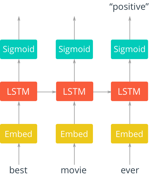
Sentiment analysis for movie reviews
Given a review about a movie written in plain english, we need to decide whether it’s positive, negative, or neutral.
This is clearly a supervised learning task, with a simple trinary label per input sample. However, we’ll need to deal with inputs of arbitrary length, provided as plain text. This is considered a challenging task for classical ML models, which used heuristics based on keywords alone.
Consider this movie review1:
"This movie was actually neither that funny, nor super witty."
The adjectives are all positive, yet they are at least partially negated. To comprehend such a sentence, it’s intuitive that we should need to keep some “state” in our head while “processing” it.
Dataset
We’ll use the torchtext package, which provides useful tools for working with textual data, and also includes some built-in datasets and dataloaders (similar to torchvision).
Our dataset will be the Stanford Sentiment Treebank (SST) dataset, which contains ~10,000 labeled movie reviews.
The label of each review is either “positive”, “neutral” or “negative”.
Working with textual inputs
Models can’t work with text: you can’t multiply a word by a weight matrix. So before each word can be fed into the model, we need to convert it into a vector.
There are a few steps involved in going from a sentence like the one above, to a sequence of
-
Tokenization: the sentence (one single string) is split into multiple smaller strings, each representing a word, punctuation mark or special token (e.g. for the start or end of a sentence).
-
Mapping the token to a vocabulary index: each token is still a string. We’ll map it to a number (just an integer). This is done simply with a huge lookup table that assigns a unique numeric ID to every possible word, punctuation mark, etc.
-
Mapping the vocabulary index to an embedding vector: For each index in our vocabulary, we’ll assign a dense
-dimensional vector to represent it. This dense vector should ideally “represent” the token (e.g. word) in some semantically meaningful way. We could use a set of pre-trained embedding vectors, or we could assign random vectors and train them together with our model.
Loading and tokenizing text samples
We’ll use the torchtext.data.Field class to take care of splitting text into unique tokens using a tokenizer called spacy. It will also build a vocabulary lookup table, which we’ll use later to convert the tokens to a numerical representation.
import torchtext.data

# torchtext Field objects parse text (e.g. a review) and create a tensor representation

# This Field object will be used for tokenizing the movie reviews text
# For this application, tokens ~= words

review_parser = torchtext.data.Field(
    sequential=True, use_vocab=True, lower=True,
    init_token='<sos>', eos_token='<eos>', dtype=torch.long,
    tokenize='spacy', tokenizer_language='en_core_web_sm'
)

# This Field object converts the text labels into numeric values (0,1,2)
label_parser = torchtext.data.Field(
    is_target=True, sequential=False, unk_token=None, use_vocab=True
)
The SST dataset we’ll use it already built into the torchtext package.
import torchtext.datasets

# Load SST, tokenize the samples and labels
# ds_X are Dataset objects which will use the parsers to return tensors
ds_train, ds_valid, ds_test = torchtext.datasets.SST.splits(
    review_parser, label_parser, root=data_dir
)

n_train = len(ds_train)
print(f'Number of training samples: {n_train}')
print(f'Number of test     samples: {len(ds_test)}')
Number of training samples: 8544
Number of test samples: 2210
Let’s print some examples from our training data:
for i in ([111, 4321, 7777, 0]):
    example = ds_train[i]
    label = example.label
    review = str.join(" ", example.text)
    print(f'sample#{i:04d} [{label:8s}]:\n > {review}\n')
sample#0111 [positive]:
> the film aims to be funny , uplifting and moving , sometimes all at once .
sample#4321 [neutral ]:
> the most anti - human big studio picture since 3000 miles to graceland .
sample#7777 [negative]:
> an ugly , revolting movie .
sample#0000 [positive]:
> the rock is destined to be the 21st century 's new ` ` conan '' and that he 's going to make a splash even greater than arnold schwarzenegger , jean - claud van damme or steven segal .
Building a vocabulary
The Field object can build a vocabulary for us, which is simply a bidirectional mapping between a unique index and a token.
We’ll only include words from the training set in our vocabulary.
review_parser.build_vocab(ds_train)
label_parser.build_vocab(ds_train)

print(f"Number of tokens in training samples: {len(review_parser.vocab)}")
print(f"Number of tokens in training labels: {len(label_parser.vocab)}")
Number of tokens in training samples: 15482
Number of tokens in training labels: 3
print(f'first 20 tokens:\n', review_parser.vocab.itos[:20], end='\n\n')first 20 tokens:
['<unk>', '<pad>', '<sos>', '<eos>', '.', 'the', ',', 'a', 'and', 'of', 'to', '-', 'is', "'s", 'it', 'that', 'in', 'as', 'but', 'film']
Note the special tokens, <unk>, <pad>, <sos> and <eos> at indexes 0-3.
These were automatically created by the tokenizer.
Let’s check whether some movie-related words exist in the vocabulary, and get their index:
for w in ['film', 'actor', 'schwarzenegger', 'spielberg']:
    print(f'word={w:15s} index={review_parser.vocab.stoi[w]}')
word=film index=19
word=actor index=492
word=schwarzenegger index=3404
word=spielberg index=715
print(f'labels vocab:\n', dict(label_parser.vocab.stoi))labels vocab:
{'positive': 0, 'negative': 1, 'neutral': 2}
Data loaders (iterators)
The torchtext package comes with Iterators, which are similar to the DataLoaders that PyTorch users are familiar with.
A key issue when working with text sequences is that each sample is of a different length (different number of words in the sentence). So, how can we work with batches of data?
BATCH_SIZE = 4

# BucketIterator creates batches with samples of similar length
# to minimize the number of <pad> tokens in the batch.
dl_train, dl_valid, dl_test = torchtext.data.BucketIterator.splits(
    (ds_train, ds_valid, ds_test), batch_size=BATCH_SIZE,
    shuffle=True, device=device)
Let’s look at a single batch.
batch = next(iter(dl_train))

X, y = batch.text, batch.label
print('X = \n', X, X.shape, end='\n\n')
print('y = \n', y, y.shape)
X =
tensor([[ 2, 2, 2, 2],
[ 56, 108, 364, 656],
[ 13, 5, 5, 776],
[ 631, 111, 270, 621],
[ 36, 19, 184, 6],
[ 23, 12, 26, 93],
[ 1949, 69, 89, 10137],
[ 193, 38, 736, 5],
[ 6, 595, 43, 1616],
[ 5115, 11, 7, 1805],
[ 941, 3010, 19, 14235],
[ 18, 45, 20, 11],
[ 32, 25, 23, 7],
[ 450, 848, 351, 11],
[ 533, 11, 51, 13313],
[ 6, 3784, 1188, 9],
[ 12, 3449, 43, 5],
[ 667, 12566, 101, 267],
[ 114, 11, 2805, 826],
[ 4848, 416, 19, 4],
[ 8, 1557, 112, 3],
[ 5625, 6, 439, 1],
[ 5, 5, 4, 1],
[ 669, 111, 3, 1],
[ 411, 167, 1, 1],
[ 55, 34, 1, 1],
[ 10, 5, 1, 1],
[ 29, 5347, 1, 1],
[ 4, 643, 1, 1],
[ 3, 13705, 1, 1],
[ 1, 6722, 1, 1],
[ 1, 12, 1, 1],
[ 1, 69, 1, 1],
[ 1, 5429, 1, 1],
[ 1, 4, 1, 1],
[ 1, 3, 1, 1]]) torch.Size([36, 4])
y =
tensor([0, 2, 1, 2]) torch.Size([4])
What are we looking at?
Our sample tensor X is of shape (sentence_length, batch_size)=(36,4). We sampled 4 sentences into this batch, each is shown here as a column with 36 tokens. The tokens are represented as indices into the vocabulary’s lookup table. Notice also that each of the sentences ends with a sequence of tokens with value 1. We can see above that the 1 token is a special token, <pad>. This is used to mark padding, i.e. unused tokens, to allow batching together sentences of different lengths.
Note also that: sentence_length will change every batch. So the input shape to the model is not fixed. This is fine for a model that expects sequences.
One strange thing here is that the sequence dimension comes first, not the batch (which is the usual pytorch convention). When we implement the model, you’ll see why it’s easier to work this way.
Model
We can now create a simple sentiment analysis model based on the RNNLayer we’ve implemented above.
The model will:
- Take an input batch of tokenized sentences.
- Compute a dense word-embedding of each token.
- Process the sentence sequentially through the RNN layer.
- Produce a
(B, 3)tensor, which we’ll interpret as class probabilities for each sentence in the batch.
Embedding layers
What is a word embedding? How do we get one?
Embeddings encode tokens as tensors in a way that maintain some semantic meaning for our task.
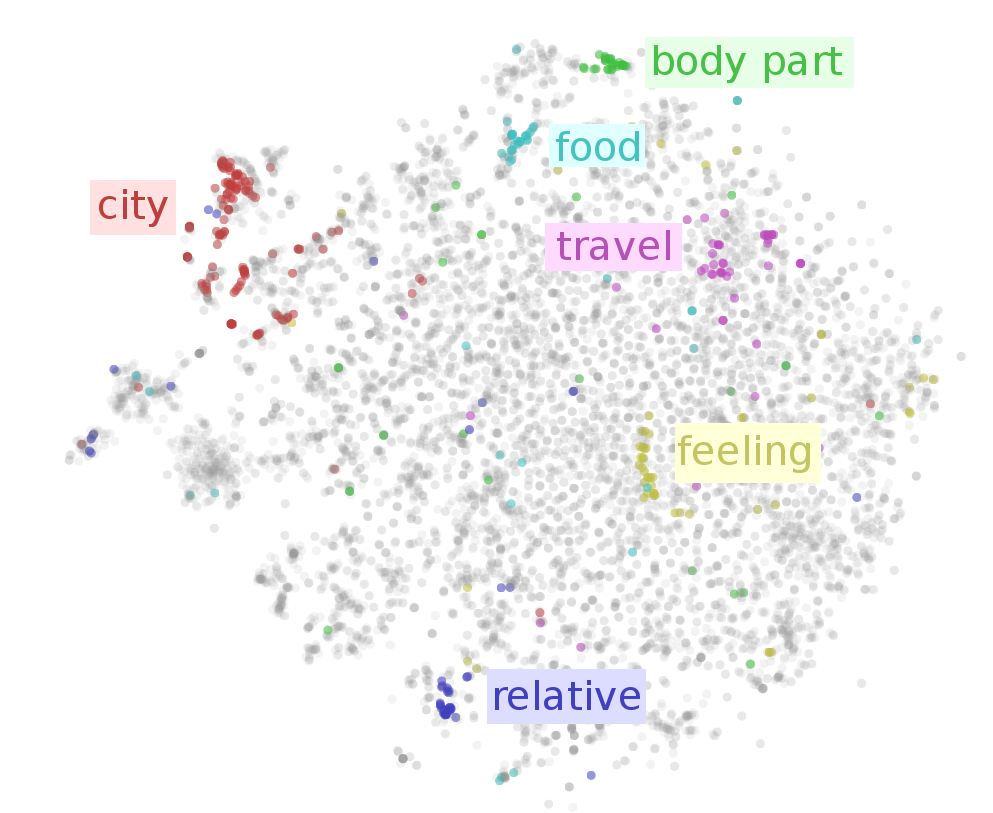
We could use a pre-trained word embedding model. There exist various general-purpose word embedding models, which all aim to learn representations which are semantically meaningful, in the sense that words that have similar meaning are “close” (e.g. in terms of cosine distance) in the embedding space.
Using a pre-trained embedding model would be a good idea in general, but here we’ll train the word embeddings together with our model. To achieve that, we’ll use a nn.Embedding layer. This is a super-simple layer. Think of it as just containing a dict, mapping from indices to randomly initialized parameter vectors, e.g. {0: nn.Parameter(torch.randn(d)), 1: ...}. When we need the embedding for a token, we’ll use the token’s index to obtain the associated vector. Over batches and epochs, each of these dense vectors will be updated via back-propagation (assuming their corresponding token existed in the input).
This will create an embedding layer that’s not general-purpose, but instead optimized for the specific task at hand (e.g. classifying movie reviews).
Here’s how to use PyTorch’s nn.Embedding:
embedding_layer = nn.Embedding(num_embeddings=5, embedding_dim=8)

token_idx = torch.randint(low=0, high=5, size=(6,))
print(token_idx)
embedding_layer(token_idx)
tensor([4, 2, 0, 0, 4, 3])
tensor([[ 0.2404, -0.5550, 0.6873, -1.0276, 0.5748, 1.3422, 1.5551, -0.9304],
[ 0.3050, -0.6279, -0.0856, 0.6240, 0.0890, -1.5827, 1.2871, -0.6937],
[-0.0246, 0.2887, 0.2568, 0.7967, 0.6089, -0.2071, 0.2202, 1.7748],
[-0.0246, 0.2887, 0.2568, 0.7967, 0.6089, -0.2071, 0.2202, 1.7748],
[ 0.2404, -0.5550, 0.6873, -1.0276, 0.5748, 1.3422, 1.5551, -0.9304],
[-0.1252, -0.3856, -0.9769, 0.5809, -0.7404, 1.2604, -1.4192, 1.0447]],
grad_fn=<EmbeddingBackward>)
Model implementation
Now that we have all the parts, it’s time to assemble. The implementation is very straightforward. Follow the comments in the code to understand how it all comes together.
class SentimentRNN(nn.Module):
    def __init__(self, vocab_dim, embedding_dim, h_dim, out_dim):
        super().__init__()

        # nn.Embedding converts from token index to dense tensor
        self.embedding = nn.Embedding(vocab_dim, embedding_dim)

        # Our own Vanilla RNN layer, without phi_y so it outputs a class score
        self.rnn = RNNLayer(in_dim=embedding_dim, h_dim=h_dim, out_dim=out_dim, phi_y=None)

        # To convert class scores to log-probability we'll apply log-softmax
        self.log_softmax = nn.LogSoftmax(dim=1)

    def forward(self, X):
        # X shape: (S, B) Note batch dim is not first!

        embedded = self.embedding(X) # embedded shape: (S, B, E)

        # Loop over (batch of) tokens in the sentence(s)
        ht = None
        for xt in embedded:           # xt is (B, E)
            yt, ht = self.rnn(xt, ht) # yt is (B, D_out)

        # Class scores to log-probability
        yt_log_proba = self.log_softmax(yt)

        return yt_log_proba
Let’s instantiate our model.
INPUT_DIM = len(review_parser.vocab)
EMBEDDING_DIM = 100
HIDDEN_DIM = 128
OUTPUT_DIM = 3

model = SentimentRNN(INPUT_DIM, EMBEDDING_DIM, HIDDEN_DIM, OUTPUT_DIM)
model
SentimentRNN(
(embedding): Embedding(15482, 100)
(rnn): RNNLayer(
(fc_xh): Linear(in_features=100, out_features=128, bias=False)
(fc_hh): Linear(in_features=128, out_features=128, bias=True)
(fc_hy): Linear(in_features=128, out_features=3, bias=True)
)
(log_softmax): LogSoftmax(dim=1)
)
Test a manual forward pass:
print(f'model(X) = \n', model(X), model(X).shape)
print(f'labels = ', y)
model(X) =
tensor([[-0.9039, -1.0806, -1.3640],
[-0.9976, -1.6040, -0.8437],
[-0.9100, -1.0781, -1.3578],
[-0.9100, -1.0781, -1.3578]], grad_fn=<LogSoftmaxBackward>) torch.Size([4, 3])
labels = tensor([0, 2, 1, 2])
How big is our model?
def count_parameters(model):
    return sum(p.numel() for p in model.parameters() if p.requires_grad)

print(f'The RNN model has {count_parameters(model):,} trainable weights.')
The RNN model has 1,577,899 trainable weights.
That’s a lot! But we used only one RNN layer. Where are all of those weights coming from?
Our custom nn.Embedding layer is actually huge, since it needs
Another thing to note that our simple forward loop ignores padding tokens, so they are processed as if they were real inputs. A proper implementation would need to skip them.
Training
We can now implement the regular pytorch-style training loop for our sentiment analysis model.
def train(model, optimizer, loss_fn, dataloader, max_epochs=100, max_batches=200):
    for epoch_idx in range(max_epochs):
        total_loss, num_correct = 0, 0
        start_time = time.time()

        for batch_idx, batch in enumerate(dataloader):
            X, y = batch.text, batch.label

            # Forward pass
            y_pred_log_proba = model(X)

            # Backward pass
            optimizer.zero_grad()
            loss = loss_fn(y_pred_log_proba, y)
            loss.backward()

            # Weight updates
            optimizer.step()

            # Calculate accuracy
            total_loss += loss.item()
            y_pred = torch.argmax(y_pred_log_proba, dim=1)
            num_correct += torch.sum(y_pred == y).float().item()

            if batch_idx == max_batches-1:
                break

        print(f"Epoch #{epoch_idx}, loss={total_loss /(max_batches):.3f}, accuracy={num_correct /(max_batches*BATCH_SIZE):.3f}, elapsed={time.time()-start_time:.1f} sec")
Running it for a few epochs on a small subset, to see that the loss starts to go down.
import torch.optim as optim

rnn_model = SentimentRNN(INPUT_DIM, EMBEDDING_DIM, HIDDEN_DIM, OUTPUT_DIM).to(device)

optimizer = optim.Adam(rnn_model.parameters(), lr=1e-3)

# Recall: LogSoftmax + NLL is equiv to CrossEntropy on the class scores
loss_fn = nn.NLLLoss()

train(rnn_model, optimizer, loss_fn, dl_train, max_epochs=4) # just a demo
Epoch #0, loss=1.106, accuracy=0.412, elapsed=4.2 sec
Epoch #1, loss=1.085, accuracy=0.409, elapsed=4.0 sec
Epoch #2, loss=1.074, accuracy=0.419, elapsed=4.2 sec
Epoch #3, loss=1.053, accuracy=0.438, elapsed=4.2 sec
Conclusions
In this post we learned how to handle sequences of inputs using deep learning models, particularly for text which has it’s own unique considerations (like tokenization and word embeddings). We saw why RNNs are a natural way to handle sequences through their hidden state, but also noticed their drawbacks, namely that they require sequential input processing and struggle with long sequences due to vanishing/exploding gradients.
We also implemented a simple vanilla RNN-based model to solve sentiment classification of movie reviews. This was just a toy solution, since we kept things as simple as possible to highlight just the core concepts. In practice, such a model would benefit from pre-trained word embeddings (e.g. GloVe or word2vec), deeper architectures, bidirectional processing, and more training. Don’t expect SotA results. :)
It’s worth re-iterating that RNNs seem to be used less and less in recent years. They are being replaced either by convolutional approaches (TCNs) or by attention-based models (transformers). Transformers in particular are becoming a dominant paradigm for NLP. I’ll try to cover both these types of models in future posts.
Despite newer approaches for modeling sequences, the core ideas covered here (recurrence, hidden state, tradeoffs between long-range modeling and trainability) remain fundamental topics and are still important considerations to keep in mind.
Footnotes
-
I found this example here: https://nlp.stanford.edu/sentiment/ ↩